


- Protocols

- Articles and Issues
- For Authors
- About
- Become a Reviewer


ROOT-ExM: Super-Resolution Imaging of Proteins in Arabidopsis Roots by Expansion Microscopy


(*contributed equally to this work) Published: Vol 16, Iss 11, Jun 5, 2026 DOI: 10.21769/BioProtoc.5707 Views: 665
Reviewed by: Shweta PanchalMalgorzata LichockaAnonymous reviewer(s)
 PDF
PDF  Ask a question
Original research article
The authors used this protocol in:
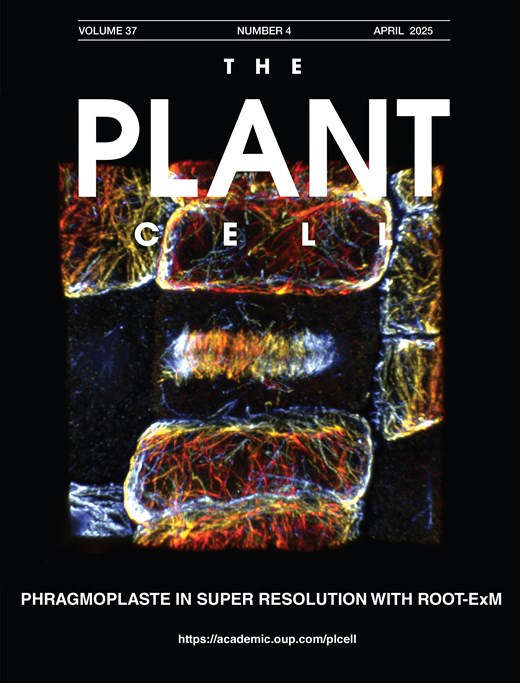
Apr 2025
Advertisement



Protocol Collections
Comprehensive collections of detailed, peer-reviewed protocols focusing on specific topics




Abstract
Conventional light microscopy is limited in resolution by the diffraction limit of light, restricting the visualization of the nanoscale organization of biomolecules. Expansion microscopy (ExM) has emerged as a powerful technique to overcome this barrier by physically expanding the specimen embedded in a swellable hydrogel without requiring specialized or high-cost imaging hardware. ExM is widely used in animal models, whereas its application to plant tissues has been challenging due to their multicellularity, in which each cell is encompassed by the rigid cell wall, which resists the expansion forces and prevents isotropic swelling. Here, we describe a robust and optimized ExM protocol specifically designed for Arabidopsis thaliana root tissues. This protocol details critical steps, including immunostaining, anchoring, gelation, denaturation, cell wall digestion, and expansion. Our method achieves an expansion factor of approximately 4.3×, enabling an effective lateral resolution of ~60 nm using a standard confocal microscope. We demonstrate the visualization of microtubules with preserved ultrastructure. This accessible protocol allows plant researchers to perform super-resolution imaging without specialized optical equipment, facilitating detailed structural analysis of plant cells.
Key features
• Expansion microscopy to break the diffraction barrier by increasing the physical distances between proteins while preserving relative spatial relationships and fluorescence signals.
• 4-fold expansion of Arabidopsis root tissues.
• 3D super-resolution imaging.
• Deep-tissue imaging thanks to optical clearing associated with expansion of hydrogel-embedded specimens.
Keywords: Expansion microscopy Super-resolution microscopy
Fluorescence microscopy
Immunostaining
Tissue clearing
Deep-tissue imaging
Plant biology
Arabidopsis thaliana root
Super-resolution microscopy
Fluorescence microscopy
Immunostaining
Tissue clearing
Deep-tissue imaging
Plant biology
Arabidopsis thaliana root
Graphical overview
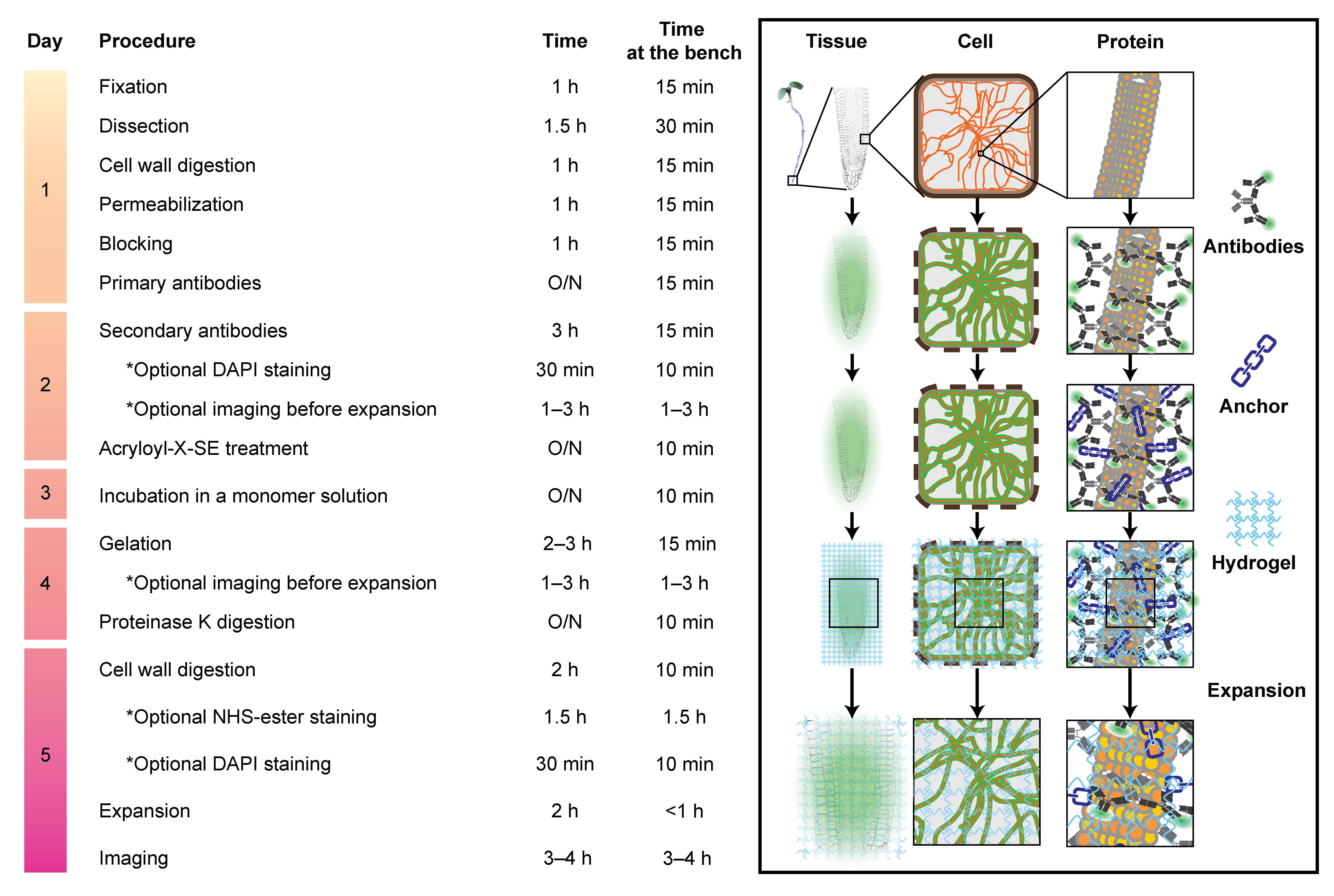
ROOT-ExM workflow and key steps. The required time indicated here includes associated procedures, such as washing.
Background
Determining molecular distribution within the cellular context is crucial for understanding biological functions. While fluorescence microscopy is a fundamental tool to fulfill this purpose in the life sciences, its resolution is, in principle, limited by the diffraction of the light. Super-resolution modalities—including stimulated emission depletion (STED) [1] and photoactivated localization microscopy (PALM) [2] or stochastic optical reconstruction microscopy (STORM) [3]—have revolutionized fluorescence microscopy by breaking this barrier, contributing to new discoveries in recent decades. However, these techniques often require expensive specialized optical setups and significant technical expertise, hindering their widespread adoption.
Imaging plant tissues presents additional unique challenges that render them optically non-ideal. Although Arabidopsis root tips are a classic model to study cell biology, physiology, and development, imaging the protein of interest within them at high resolution is difficult due to (i) cylindrical geometry and low adhesiveness of the root tissue, which often prevents close contact of the cell of interest with coverslips, (ii) refractive index mismatches caused by heterogeneous structures in plant cells, such as the cell wall, cytoplasm, and vacuole [4,5], and (iii) light scattering by the multi-layered organization of such cells. Particularly, routinely studied root epidermal cells in the meristematic zone are obscured by the lateral root cap cells. These factors collectively result in reduced signal-to-noise ratios and spatial resolution [6–9].
Expansion microscopy (ExM), a distinct paradigm for achieving super-resolution imaging first reported in 2015, offers a robust solution to these issues [10]. The principle of ExM is to physically expand the specimen and increase spatial distance between molecules. Thus, ExM enables super-resolution imaging even with conventional diffraction-limited microscopes. In ExM, specific biomolecules such as proteins are chemically modified with the so-called anchor. Subsequently, a swellable polyelectrolyte gel is synthesized throughout the biological sample, while the modified biomolecules can covalently bind to the hydrogel matrix. After gel polymerization, the embedded sample is treated by enzymatic digestion or heat- and detergent-induced denaturation, which is the so-called mechanical homogenization. This loosens adhesiveness derived from intra- and intermolecular interactions and creates appropriate uniformity in mechanical properties of the biological sample, which resists expansion, so that the resulting sample expands isotropically through dialysis in distilled water. As fluorophores are adequately preserved due to their stability to digestion or denaturation, the protein of interest can be localized at super-resolution after expansion. The expansion process also results in significant optical clearing and homogenizes the refractive index of the sample to match that of water. This makes ExM particularly advantageous for imaging in complex plant tissues.
Here, we present a step-by-step protocol for applying ExM to Arabidopsis root tips to achieve robust and reproducible super-resolution imaging of proteins of interest, which utilizes acryloyl-X, SE for anchoring, and sodium acrylate/acrylamide/N,N′-methylenebisacrylamide for the gel matrix. Our ROOT-ExM protocol is based on the pre-expansion staining protein-retention ExM (proExM) previously described in mammalian cells [11] and includes critical optimizations for plant tissues [12]. Most notably, we introduce a cell wall digestion step to overcome the mechanical rigidity imposed by the cell wall, allowing for uniform isotropic expansion. This protocol covers all steps from sample preparation and immunostaining to anchoring, gelation, mechanical homogenization, expansion, and image analysis. The resulting root tip undergoes an approximate 4.3-fold linear expansion and exhibits a water-matching refractive index, enabling super-resolution and deep-tissue imaging.
Materials and reagents
Biological materials
1. Arabidopsis thaliana ecotype Col-0: wild type
Note: Other ecotypes or transgenic lines expressing fluorescent proteins can also be used.
Reagents
1. Murashige and Skoog (MS) medium including vitamins powder (Duchefa Biochemie, catalog number: M0222.0050), storage temperature: 4 °C
2. Sucrose (Sigma-Aldrich, catalog number: 84100), storage temperature: room temperature (RT)
3. MES [2-(N-morpholino)ethanesulfonic acid] (Euromedex, catalog number: EU0033-A), storage temperature: RT
4. Plant agar (Duchefa Biochemie, catalog number: P1001.1000), storage temperature: RT
5. Potassium hydroxide (KOH) (Sigma-Aldrich, catalog number: P5958), storage temperature: RT
6. PIPES [piperazine-N,N′-bis(2-ethanesulfonic acid)] (Sigma-Aldrich, catalog number: P6757), storage temperature: RT
7. EGTA [ethylene glycol-bis(2-aminoethylether)-N,N,N′,N′-tetraacetic acid] (Sigma-Aldrich, catalog number: E4378), storage temperature: RT
8. Magnesium sulfate (MgSO4·7H2O) (Euromedex, catalog number: P027-A), storage temperature: RT
9. Paraformaldehyde solution, 16% (Ted Pella, catalog number: 18505), storage temperature: 4 °C
10. Driselase (Sigma-Aldrich, catalog number: D9515-5G), storage temperature: -20 °C
11. Macerozyme R-10 (Duchefa Biochemie, catalog number: M8002.0005), storage temperature: 4 °C
12. DMSO (dimethyl sulfoxide) (Sigma-Aldrich, catalog number: D8418), storage temperature: RT
13. DMSO, anhydrous (Invitrogen, catalog number: D12345), storage temperature: RT
14. IGEPAL CA-630 (Sigma-Aldrich, catalog number: I3021), storage temperature: RT
15. Bovine serum albumin (BSA) (Euromedex, catalog number: 1035-70-C), storage temperature: 4 °C
16. DAPI (4',6-diamidino-2-phenylindole) dihydrochloride (Sigma-Aldrich, catalog number: D8417-1MG), storage temperature: 4 °C
17. Acryloyl-X, SE [6-((acryloyl)amino)hexanoic acid, succinimidyl ester] (Thermo Fisher Scientific, catalog number: A20770), storage temperature: -20 °C
18. Sodium acrylate (Combi-Blocks, catalog number: QC-1489), storage temperature: 4 °C
19. Proteinase K, ≥30 units/mg (Sigma-Aldrich, catalog number: P2308-25MG), storage temperature: -20 °C
20. PBS (10×), pH 7.4 (Thermo Fisher Scientific, catalog number: 70011044), storage temperature: RT
21. 40% acrylamide solution (Sigma-Aldrich, catalog number: A4058-100ML), storage temperature: 4 °C
22. 2% N,N′-Methylenebisacrylamide solution (Sigma-Aldrich, catalog number: M1533-25ML), storage temperature: 4 °C
23. 4-Hydroxy-TEMPO (Sigma-Aldrich, catalog number: 176141-1G), storage temperature: 4 °C
24. TEMED (N,N,N′,N′-Tetramethylethylenediamine) (Sigma-Aldrich, catalog number: T7024-25ML), store at RT or 4 °C
25. Ammonium persulfate (APS) (Sigma-Aldrich, catalog number: A3678-25G), store at RT or 4 °C
26. Sodium chloride (NaCl) (Sigma-Aldrich, catalog number: S7653), storage temperature: RT
27. Tris base (Sigma-Aldrich, catalog number: 252859), storage temperature: RT
28. Ethylenediaminetetraacetic acid tetrasodium salt dihydrate (EDTA) (Sigma-Aldrich, catalog number: ED4SS), storage temperature: RT
29. Hydrochloric acid (HCl) (Sigma-Aldrich, catalog number: 258148), storage temperature: RT
30. Sodium hydroxide (NaOH) (Euromedex, catalog number: 2020), storage temperature: RT
31. Triton X-100 (Sigma-Aldrich, catalog number: T9284), storage temperature: RT
32. Guanidine hydrochloride (Sigma-Aldrich, catalog number: G3272), storage temperature: RT
33. Sodium bicarbonate (NaHCO3) (Sigma-Aldrich, catalog number: S6297), storage temperature: RT
34. 52.5% nitric acid (HNO3) (Prolabo, catalog number: 20420.291), storage temperature: RT
35. Ethanol (Fisher Scientific, catalog number: E-0650DF-17), storage temperature: RT
36. APTES [(3-Aminopropyl)triethoxysilane] (Sigma-Aldrich, catalog number: A3648), storage temperature: 4 °C
37. Mouse anti-α-tubulin monoclonal primary antibody (Sigma-Aldrich, catalog number: T5168) (1:500 dilution)
38. Donkey anti-mouse IgG secondary antibody conjugated with Alexa Fluor 488 (Abcam, catalog number: ab150105) (1:500 dilution), storage temperature: -20 °C (stock aliquots) or 4 °C for 4 weeks (thawed aliquots)
39. Goat anti-mouse IgG secondary antibody conjugated with Alexa Fluor 594 (Invitrogen, catalog number: A-11005) (1:500 dilution), storage temperature: -20 °C (stock aliquots) or 4 °C for 4 weeks (thawed aliquots)
40. NHS ester-ATTO647 (Sigma-Aldrich, catalog number: 07376), storage temperature: -20 °C
Note: Other fluorophore-conjugated NHS esters can also be used.
Solutions
1. 10 M KOH (see Recipes)
2. 1/2× MS solid media (see Recipes)
3. 4/3× microtubule stabilizing buffer (MTSB) (see Recipes)
4. MTSB (see Recipes)
5. Fixation solution (see Recipes)
6. Cell wall digestion solution I (see Recipes)
7. Permeabilization solution (see Recipes)
8. Blocking buffer (see Recipes)
9. DAPI solution (1,000×) (see Recipes)
10. PBS (see Recipes)
11. Acryloyl-X, SE stock solution (100×) (see Recipes)
12. 4-Hydroxy-TEMPO stock solution (50×) (see Recipes)
13. TEMED stock solution (50×) (see Recipes)
14. APS stock solution (50×) (see Recipes)
15. Sodium acrylate solution (see Recipes)
16. Monomer stock solution (see Recipes)
17. Gelation solution (see Recipes)
18. 1 M Tris (pH 8.0) (see Recipes)
19. 0.5 M EDTA (see Recipes)
20. Protein digestion buffer (see Recipes)
21. Proteinase K stock solution (100×) (see Recipes)
22. Protein digestion solution (see Recipes)
23. Cell wall digestion solution II (see Recipes)
24. NHS ester labeling buffer (see Recipes)
25. NHS ester stock solution (see Recipes)
26. NHS ester labeling solution (see Recipes)
Recipes
Caution: This protocol involves the use of chemicals classified as carcinogenic, mutagenic, and reprotoxic (CMR), such as paraformaldehyde and acrylamide. Therefore, appropriate personal protective equipment should be worn, and if necessary, all manipulations involving CMRs must be performed under a fume hood.
1. 10 M KOH
| Reagent | Final concentration | Amount |
|---|---|---|
| KOH | 10 M | 28.05 g |
| Ultrapure water | n/a | Make up to 50 mL |
Store in a plastic bottle/tube at RT
2. 1/2× MS solid media
| Reagent | Final concentration | Amount |
|---|---|---|
| MS powder | 1/2× | 2.2 g |
| Sucrose | 1% | 10 g |
| MES | 2.5 mM | 0.49 g |
| 10 M KOH | n/a | Adjust the pH to 5.8 |
| Plant agar | 0.8% | 8 g |
| Ultrapure water | n/a | Make up to 1 L |
Autoclave at 110 °C for 30 min and dispense 50 mL per 12 cm × 12 cm square Petri dish. Store the solidified agar media at 4 °C.
3. 4/3× MTSB
| Reagent | Final concentration | Amount |
|---|---|---|
| PIPES | 66.67 mM | 5.04 g |
| EGTA | 6.67 mM | 0.63 g |
| MgSO4·7H2O | 6.67 mM (MgSO4) | 0.41 g |
| KOH | n/a | Adjust the pH to 7 |
| Ultrapure water | n/a | Make up to 250 mL |
Autoclave at 110 °C for 30 min. Store at 4 °C.
4. MTSB
| Reagent | Final concentration | Amount |
|---|---|---|
| PIPES | 50 mM | 15.12 g |
| EGTA | 5 mM | 1.89 g |
| MgSO4·7H2O | 5 mM (MgSO4) | 1.23 g |
| KOH | n/a | Adjust the pH to 7 |
| Ultrapure water | n/a | Make up to 1 L |
Autoclave at 110 °C for 30 min. Store at 4 °C.
5. Fixation solution
| Reagent | Final concentration | Amount |
|---|---|---|
| 16% Paraformaldehyde solution | 4% (v/v) | 10 mL (1 ampoule) |
| 4/3× MTSB | 1× | 30 mL |
Note: This solution should be freshly prepared for each experiment. However, the rest can be stored at 4 °C for a week or at -20 °C for a month.
6. Cell wall digestion solution I
| Reagent | Final concentration | Amount per reaction |
|---|---|---|
| Driselase | 2% (w/v) | 4 mg |
| MTSB | 1× | 200 μL |
Centrifuge at 1,000× g for 1 min and use the supernatant.
Note: This solution should be freshly prepared for each experiment.
7. Permeabilization solution
| Reagent | Final concentration | Amount per reaction |
|---|---|---|
| DMSO | 10% (v/v) | 20 μL |
| IGEPAL CA-630 | 3% (v/v) | 6 μL |
| MTSB | 1× | 174 μL |
Note: This solution should be freshly prepared for each experiment.
8. Blocking buffer
| Reagent | Final concentration | Amount per reaction |
|---|---|---|
| BSA | 3% (w/v) | 6 mg |
| MTSB | 1× | 200 μL |
Note: This solution should be freshly prepared for each experiment.
9. DAPI solution (1,000×)
| Reagent | Final concentration | Amount |
|---|---|---|
| DAPI dihydrochloride | 2 mg/mL | 1 mg |
| Ultrapure water | n/a | 0.5 mL |
Prepare 10 μL aliquots in 0.5 mL tubes and store at -20 °C.
10. PBS
| Reagent | Final concentration | Amount |
|---|---|---|
| PBS (10×) | 1× | 5 mL |
| Sterilized ultrapure water | n/a | 45 mL |
Store at 4 °C.
11. Acryloyl-X, SE stock solution (100×)
| Reagent | Final concentration | Amount |
|---|---|---|
| Acryloyl-X, SE | 10 mg/mL | 5 mg |
| DMSO | n/a | 0.5 mL |
Prepare 10 μL aliquots in 0.5 mL tubes and store at -20 °C.
12. 4-Hydroxy-TEMPO stock solution (50×)
| Reagent | Final concentration | Amount |
|---|---|---|
| 4-Hydroxy-TEMPO | 0.5% (w/w) | 50 mg |
| Ultrapure water | n/a | 10 mL |
Prepare 50 μL aliquots in 0.5 mL tubes and store at -20 °C.
13. TEMED stock solution (50×)
| Reagent | Final concentration | Amount |
|---|---|---|
| TEMED | 10% (v/v) | 1 mL |
| Ultrapure water | n/a | 9 mL |
Prepare 50 μL aliquots in 0.5 mL tubes and store at -20 °C.
14. APS stock solution (50×)
| Reagent | Final concentration | Amount |
|---|---|---|
| APS | 10% (w/w) | 1 g |
| Ultrapure water | n/a | 10 mL |
Prepare 50 μL aliquots in 0.5 mL tubes and store at -20 °C.
15. Sodium acrylate solution
| Reagent | Final concentration | Amount |
|---|---|---|
| Sodium acrylate | 35.5% (w/w) | 2.2 g |
| Ultrapure water | n/a | 4 mL |
Critical: Check the purity by the color of the solution. It should be clear, slightly yellowish (Figure 1). If this is not the case, we recommend purchasing a new bottle of sodium acrylate.
Note: Make this immediately before preparing a monomer stock solution. The resulting volume will be approximately 4.5 mL.
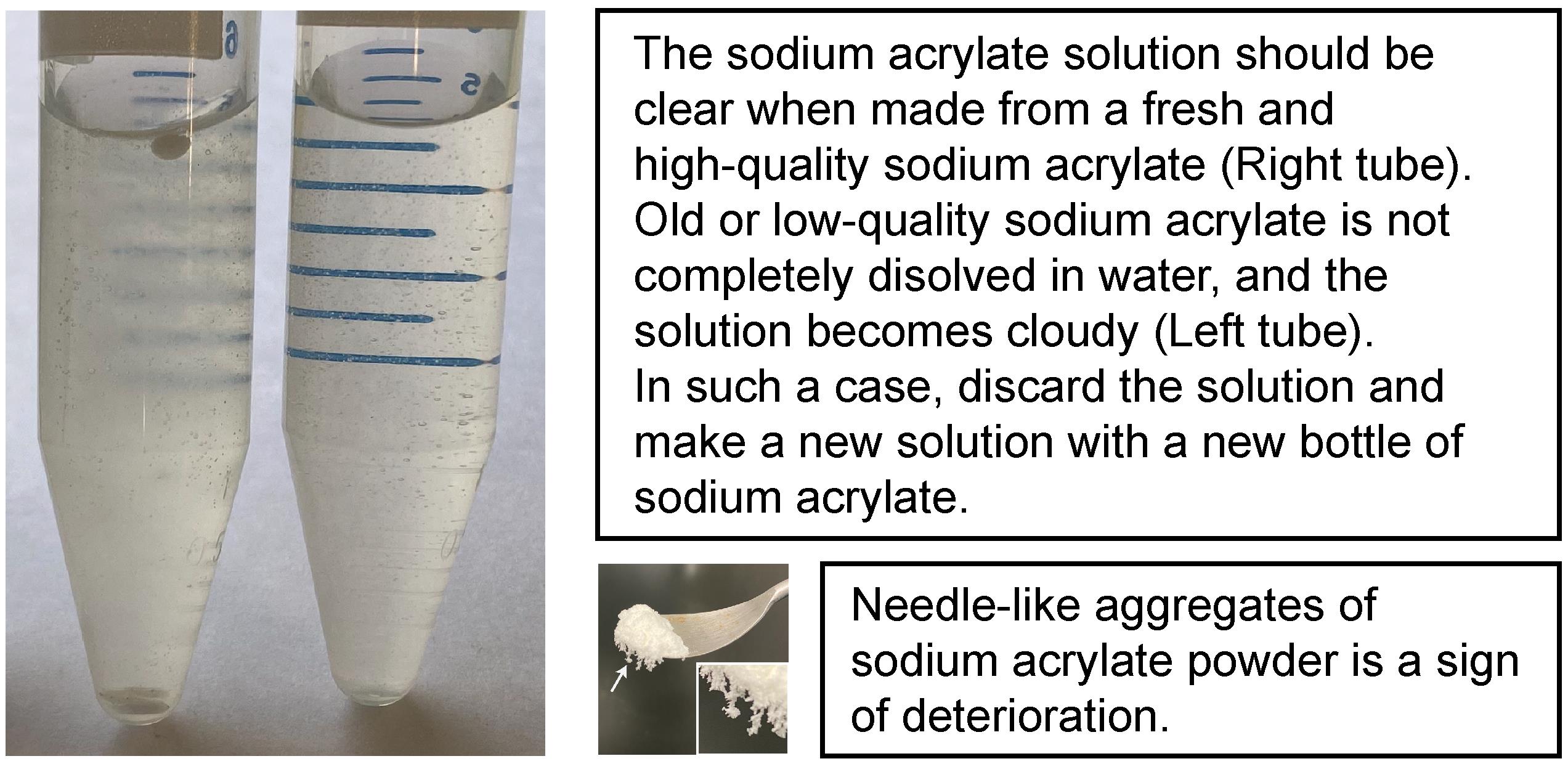
Figure 1. Quality check of sodium acrylate
16. Monomer stock solution
| Reagent | Final concentration | Amount |
|---|---|---|
| Sodium acrylate solution | 8.5% (8%) (w/w) | 4.5 mL |
| 40% Acrylamide solution | 2.1% (2%) (w/v) | 1 mL |
| 2% N,N′-Methylenebisacrylamide solution | 0.16% (0.15%) (w/v) | 1.5 mL |
| NaCl | 2.13 M (2 M) | 2.34 g |
| PBS (10×) | 1.06× (1×) | 2 mL |
| Ultrapure water | n/a | Make up to 18.8 mL |
Prepare 470 μL aliquots in 0.5 mL tubes and store at -20 °C.
Note: The concentration of each component will slightly decrease in a gelation solution with the addition of 4-Hydroxy-TEMPO, TEMED, and APS. These concentrations are shown in the brackets. One aliquot is generally used for two coverslips.
17. Gelation solution
| Reagent | Final concentration | Amount per reaction |
|---|---|---|
| Monomer solution | see above | 188 μL |
| 4-Hydroxy-TEMPO stock solution | 0.01% (w/w) | 4 μL |
| TEMED stock solution | 0.2% (v/v) | 4 μL |
| APS stock solution | 0.2% (w/w) | 4 μL |
Note: 4-Hydroxy-TEMPO, TEMED, and APS should be added sequentially in this order. Mix thoroughly after each addition. This solution should be prepared on ice immediately before the gelation step.
18. 1 M Tris (pH 8)
| Reagent | Final concentration | Amount |
|---|---|---|
| Tris base | 1 M | 12.11 g |
| HCl | n/a | Adjust the pH to 8 |
| Ultrapure water | n/a | Make up to 100 mL |
Store at RT.
19. 0.5 M EDTA
| Reagent | Final concentration | Amount |
|---|---|---|
| EDTA·4Na·2H2O | 0.5 M (EDTA) | 20.81 g |
| HCl | n/a | Adjust the pH to 8 |
| Ultrapure water | n/a | Make up to 100 mL |
Store at RT.
20. Protein digestion buffer
| Reagent | Final concentration | Amount |
|---|---|---|
| 1 M Tris (pH 8) | 50 mM | 5000 μL |
| 0.5 M EDTA | 2.5 mM | 500 μL |
| Triton X-100 | 0.5% (v/v) | 500 μL |
| Guanidine hydrochloride | 0.8 M | 7.64 g |
| Ultrapure water | n/a | Make up to 100 mL |
Prepare 10 mL aliquots and store at -20 °C.
Note: After thawing, the protein digestion buffer can be stored at 4 °C.
21. Proteinase K stock solution (100×)
| Reagent | Final concentration | Amount |
|---|---|---|
| Proteinase K, ≥30 units/mg | ≥800 units/ml | 25 mg |
| Ultrapure water | n/a | 937.5 μL |
Prepare 10 μL aliquots in 0.5 mL tubes and store at -20 °C.
22. Protein digestion solution
| Reagent | Final concentration | Amount per reaction |
|---|---|---|
| Proteinase K stock solution (100×) | ≥8 units/ml | 5 μL |
| Protein digestion buffer | n/a | 495 μL |
Note: This solution should be freshly prepared for each experiment.
23. Cell wall digestion solution II
| Reagent | Final concentration | Amount per reaction |
|---|---|---|
| Driselase | 2% | 10 mg |
| Macerozyme R-10 | 0.5% | 2.5 mg |
| PBS | 1× | 500 μL |
Centrifuge at 1,000× g for 1 min and use the supernatant.
Note: This solution should be freshly prepared for each experiment.
24. NHS ester labeling buffer
| Reagent | Final concentration | Amount per reaction |
|---|---|---|
| NaHCO3 | 100 mM | 0.42 g |
| HCl (0.1 or 1 M) | n/a | Adjust the pH to 8 |
| Ultrapure water | n/a | 50 mL |
Store at -20 °C.
Note: CO2 loss during storage leads to a gradual rise in pH. Keep the bottle tightly sealed with minimal headspace. It is highly recommended to verify the pH immediately before use, especially after prolonged storage.
25. NHS ester stock solution (100×)
| Reagent | Final concentration | Amount |
|---|---|---|
| NHS ester dye | 2 mg/mL | 1 mg |
| DMSO, anhydrous | n/a | 500 μL |
Prepare 10 μL aliquots in 0.5 mL tubes and store at -20 °C. Thawed aliquots can be stored at 4 °C for 4 weeks.
26. NHS ester labeling solution
| Reagent | Final concentration | Amount per reaction |
|---|---|---|
| NHS ester labeling buffer | n/a | 990 μL |
| NHS ester stock solution (100×) | 20 μg/mL | 10 μL |
Note: This solution should be freshly prepared for each experiment.
Laboratory supplies
1. Corning® BioCoat® Poly-D-Lysine 12 mm #1 German glass coverslip (Corning, catalog number: 354086)
Note: Homemade Poly-D-Lysine-coated round coverslips (ø 12 or 18 mm) can also be used.
2. Hydrophobic barrier pen (Vector Laboratories, catalog number: H-4000)
3. Square Petri dish, 120 × 120 × 17 mm (Greiner Bio-One, catalog number: 688102)
4. Round Petri dish, 100 × 20 mm (Greiner Bio-One, catalog number: 664102)
5. 6-well cell culture plate (Thermo Fisher Scientific, catalog number: 140675)
6. Tweezer (Hammacher, catalog number: HWC110-10)
7. Tweezer style 7 (Dumont, catalog number: 0304-7-PO)
8. Grease (Dow Corning Toray, catalog number: Dow Corning® High Vacuum Grease)
9. Glass microscope slide (Epredia, catalog number: AG00000112E04CML21
10. 18 × 18 mm coverslip (Knittel, catalog number: VD11818Y1A.01)
11. Razor blade (Accutec, catalog number: AGBL-7032-0000)
12. Parafilm (Amcor, catalog number: PM-996)
13. Aluminum foil (Alujet, catalog number: AP326)
Equipment
1. Stereomicroscope (Leica, model: MZ16F)
2. Confocal laser-scanning microscope (Carl Zeiss, model: LSM 880)
3. Dry objective lens, 10× (Carl Zeiss, model: Objective Plan-Apochromat 10×/0.45 M27)
4. Dry objective lens, 20× (Carl Zeiss, model: Objective Plan-Apochromat 20×/0.8 M27
5. Water-immersion objective lens, 40× (Carl Zeiss, model: Objective W Plan-Apochromat 40×/1.0 DIC M27)
Software and datasets
1. ZEN black 2.3 SP1 FP3 software (Carl Zeiss, version 14.0)
2. Fiji/ImageJ (version 2.16.0/1.54p) (https://imagej.net/software/fiji/)
3. All computational analyses were performed using Python 3.10.19 with SimpleITK-SimpleElastix (v2.0.0rc2.dev910) on Windows 10/11 (64-bit). The exact computational environment is archived in a public repository to ensure reproducibility (https://src.koda.cnrs.fr/bic-tai/expansion_analysis_protocol).
Procedure
Note: There is no need for shaking or repetitive pipetting during washing processes in the protocol. To wash the sample, remove the old solution, add a new solution, let it stand for the indicated time, and repeat the procedure for the specified number of times.
A. Sample preparation
1. Grow Arabidopsis plants on vertically placed 1/2× MS solid media for 5 days.
2. Incubate the 5-day-old seedlings in a 6-well cell culture plate containing 4 mL of the fixation solution for 45 min at 23 °C.
Note: The fixation solution should be prepared and dispensed into a well of the 6-well plate under the fume hood, but it is important to turn it off while transferring the seedlings into the wells; otherwise, the root tip will be severely damaged by the air flow.
3. Remove the fixation solution and wash three times for 5 min each with 4 mL of MTSB at RT.
Pause point: Fixed seedlings can be stored in MTSB overnight at 4 °C.
4. Wash with ultrapure water once for 5 min.
5. Create a cutting space in a microscope slide by dropping 10–100 μL of ultrapure water (Figure 2).
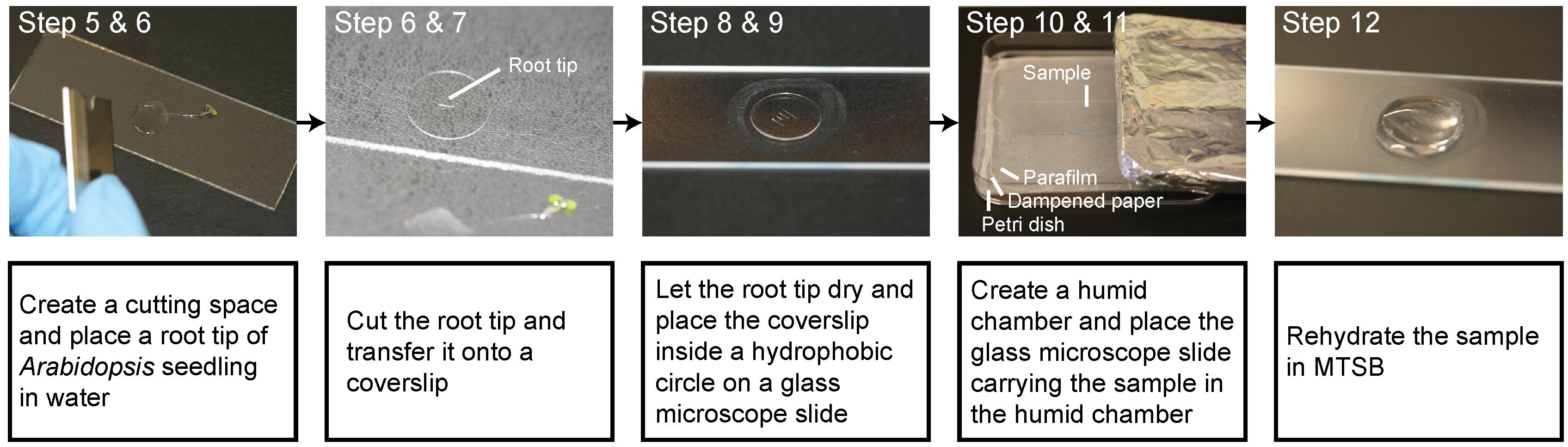
Figure 2. Preparation of the biological sample
6. Cut the Arabidopsis root tip (approximately 5 mm) with a razor blade in the cutting space and transfer the root tip onto a Poly-D-Lysine-coated 12 mm round coverslip using a precision tweezer.
Note: Several root tips (e.g., 1–5) can be placed on one coverslip. The root tip can easily detach from the coverslip during the procedure. Prepare several coverslips each time to make sure to have at least two roots after expansion.
7. Let the root tip dry for 1 h at RT to attach to the coverslip.
Pause point: Dried samples can be stored for a few weeks at -20 °C. Place the coverslip carrying the root sample inside a well of a 12- or 24-well cell culture plate and put this multi-well plate in a freezer. When using the stored sample, it needs to be re-dried for 10–15 min before proceeding to rehydration (step 12).
Note: Wild-type Arabidopsis root tips can be stored for a few weeks, but Arabidopsis transgenic lines expressing the protein tagged with fluorescent proteins should be kept only for two weeks; otherwise, the fluorescence will be reduced. We recommend proceeding immediately to the next step if possible.
8. Draw a circle with a hydrophobic barrier pen on a microscope slide. The diameter should be slightly larger than the round coverslip.
9. Place the coverslip carrying the root tip inside the hydrophobic circle on the microscope slide.
10. Create a humid chamber: cover the bottom of a square Petri dish with a piece of paper dampened with ultrapure water and place a square cut of parafilm on the top of it. Squeeze out the bubbles to obtain a flat surface.
11. Transfer the microscope slide to the humid chamber.
Note: Alternatively, place the coverslip into a well of a 24-well cell culture plate, so that it can be used as the humid incubation chamber.
B. Immunostaining
12. Pipette 200 μL of MTSB onto the coverslip and rehydrate the sample for 5 min at RT. Make sure the coverslip is in MTSB and does not float.
13. Remove MTSB and incubate with 200 μL of cell wall digestion solution I for 40 min at 23 °C.
14. Wash four times for 5 min each with 200 μL of MTSB at RT.
15. Incubate with 200 μL of the permeabilization solution for 30 min at 23 °C.
16. Wash four times for 5 min each with 200 μL of MTSB at RT.
17. Incubate with 200 μL of the blocking solution for 1 h at 23 °C.
18. Replace the blocking solution with 150 μL of the primary antibody solution at the appropriate concentration in the blocking solution and incubate overnight at 4 °C or for 2 h at 37 °C.
19. Wash four times for 5 min each with 200 μL of MTSB at RT.
20. Incubate with 150 μL of the secondary antibody solution at the appropriate concentration in blocking buffer for 2 h at 30 °C.
21. Wash four times for 5 min each with 200 μL of MTSB at RT.
Pause point: Immunostained samples can be stored for a few days at 4 °C in the dark.
22. (Optional) Mix anti-fluorescent protein nanobodies at the appropriate concentration in the blocking buffer and incubate the sample in this mixture for 2 h at 30 °C. Then, wash four times for 5 min each with 200 μL of MTSB at RT.
Note: This enhances the fluorescence signal coming from transgenic lines expressing fluorescent proteins. We routinely use the nanobody conjugated to fluorescent dyes (ChromoTek GFP- or RFP-Boosters, Proteintech).
23. (Optional) Perform additional staining with DAPI. We usually incubate the sample with 150 μL of 2 μg/mL DAPI in MTSB for 5 min at RT. Then, we wash the sample four times for 5 min each with 200 μL of MTSB at RT.
Note: This facilitates tissue recognition and makes it easier to identify the same cell before and after expansion.
24. (Optional) Acquire pre-expansion fluorescence images of the root cells if the calculation of expansion factors and evaluation of distortions are planned based on the fluorescence image. Place the coverslip on an appropriate imaging chamber with the glass side facing up to observe the sample using an upright microscope (see Figure 3 as an example). Capture fluorescence images using a confocal laser scanning microscope equipped with 20× dry and/or 40× water-immersion objectives.
Notes:
1. This is highly recommended, as the precise expansion factor varies from sample to sample. Pre-expansion imaging is also possible immediately after gelation (at step 34). Alternatively, the approximate expansion factor can be evaluated by measuring the gel size before and after expansion.
2. Depending on the availability of the microscopy system, an inverted microscope equipped with a long working distance objective can also be used.

Figure 3. Pre-expansion pre-gelation imaging
25. Put the coverslip back inside the hydrophobic circle on the microscope slide.
Note: If grease was used during imaging, remove it from the coverslip.
C. Anchoring
26. Rinse twice with 200 μL of PBS at RT.
27. Dilute Acryloyl-X, SE stock solution 1:100 in PBS and incubate the sample in 200 μL of this solution for 20–24 h at RT in the dark.
28. Wash twice for 5 min each with 200 μL of PBS at RT.
D. Gelation and mechanical homogenization
29. Thaw a 470 μL aliquot of the monomer stock solution on ice and add 10 μL of 4-Hydroxy-TEMPO to it. Incubate the sample in 150–200 μL of this mixture overnight at 4 °C in the dark.
Note: The incubation can be shortened to a minimum of 6 h; however, do not reduce the time further, as the sample may rupture during the expansion process. Do not add TEMED or APS at this step.
30. Prepare the gelation solution on ice (200 μL per coverslip). Replace the monomer stock solution added in step 29 with 200 μL of the gelation solution. Incubate the sample for 25 min on ice in the dark.
Note: One aliquot of the monomer stock solution can be used to complete the polymerization of two gels. Take 188 or 376 μL (for 1 or 2 coverslips, respectively) of the monomer stock solution to a new tube to prepare the gelation solution for this step, while the rest can be kept on ice and used at step 30.
31. Create a new humid chamber.
32. Prepare the gelation solution on ice (35 μL per coverslip), pipette a 35 μL droplet of the fresh gelation solution onto the parafilm inside the new humid chamber, and place the coverslip carefully on the droplet with the root side down (Figure 4). Close the lid of the chamber and incubate for 2 h at 37 °C in the dark.
Note: When using an 18 mm round coverslip, apply a 55 μL droplet of the fresh gelation solution.
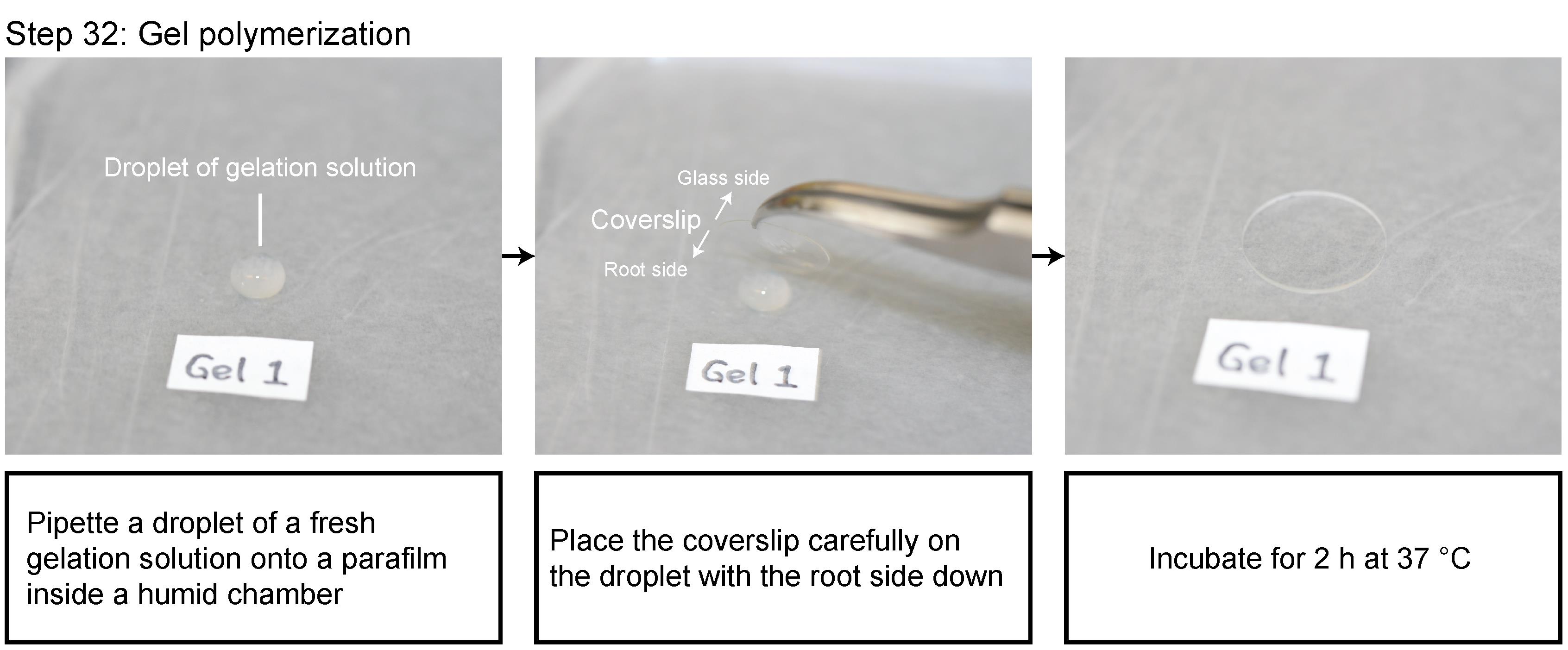
Figure 4. Gel polymerization
33. After gel polymerization, carefully detach the coverslip/gel complex from the parafilm using tweezers.
Note: Remove the excess gel around the root tip using the razor blade, and record the size of the cut gel if the calculation of the approximate expansion factor is planned based on the gel size.
34. (Optional) Acquire pre-expansion fluorescence images (Figure 5).
Note: Keep the gel in the humid chamber except when observed under the microscope to avoid drying. Avoid contact of the gel with water, as it will start to expand. In this case, DAPI cannot be used or imaged to visualize nuclei.
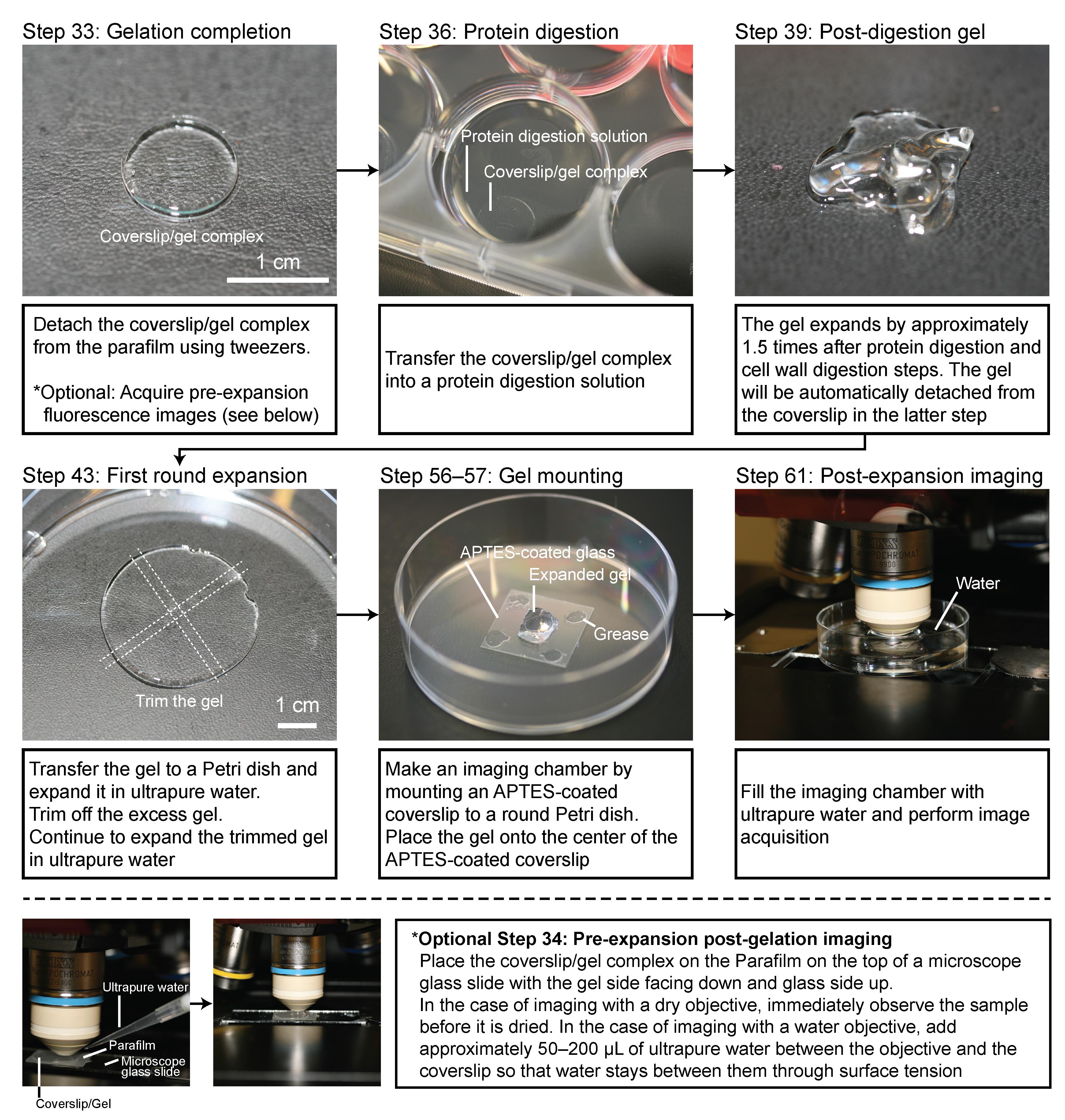
Figure 5. Post-gelation procedures
35. For each coverslip/gel complex, prepare the protein digestion solution by adding 10 μL of proteinase K stock solution to 990 μL of the protein digestion buffer and dispense it into a new individual well of the 6-well plate.
36. Transfer the coverslip/gel complex to the 6-well plate containing the protein digestion solution (Figure 5). Incubate overnight at 23 °C in the dark.
Note: This step can be shortened to 1 h by incubating the sample at 37 °C.
37. Wash twice for 5 min each with 1,000 μL of PBS at RT.
Pause point: The gel can be stored in PBS for a few days at 4 °C in the dark.
38. Incubate the sample in 500 μL of cell wall digestion solution II for 2 h at 30 °C.
39. Wash twice for 5 min each with 1,000 μL of PBS at RT or directly proceed to step 41.
Pause point: After washing with PBS, the gel can be stored in PBS for a few days at 4 °C in the dark.
Note: The gel starts to expand during the homogenization steps, and it may roll up or become ruffled while some parts of the gel stick to the coverslip (Figure 5). This is normal, and the gel itself will naturally come away from the coverslip and flatten during the subsequent step. Otherwise, the gel can be trimmed away from the coverslip using the razor blade.
E. Expansion
40. (Optional) Perform additional staining with NHS ester. Incubate the gel with 1,000 μL of NHS ester labeling solution for 1.5 h at RT under gentle shaking. Then, wash the sample three times for 5 min each with 1,000 μL of PBS at RT.
Note: This provides the cellular context (Figure 6). DAPI can be added to the NHS ester labeling solution.
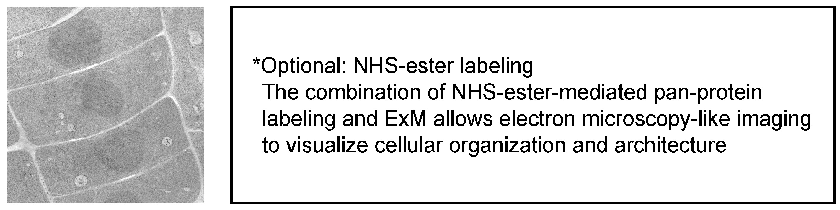
Figure 6. NHS ester labeling
41. Gently transfer the gel to a round Petri dish (ø 100 mm).
42. Add ultrapure water in excess (e.g., 20 mL) and incubate for 20 min at RT.
43. Remove the water and trim the gel to the minimum size necessary using coverslips (if necessary, under a stereomicroscope) (Figure 5).
Note: At this stage, the roots are still visible, but it will be hard to identify them after the complete expansion of the sample. The gel can be trimmed even before expansion using the razor blade (see step 33). However, the pre-expansion gel is quite sticky, and it is easier to trim at this step. Coverslips work better to cut gels after the start of expansion than the razor blade.
44. (Optional) Perform additional staining with DAPI. In the experiments presented here, we incubated the gel with 500 μL of 2 μg/mL DAPI in ultrapure water for 30 min at RT.
Note: This facilitates locating samples and is highly recommended, as the root tip will be almost invisible in the brightfield view after complete expansion. However, if DAPI staining is performed at step 40, there is no need to perform this step.
45. Add ultrapure water in excess again and incubate for 20 min at RT. Renew the ultrapure water and repeat this step three or more times. The sample should be fully expanded and optically cleared.
F. Preparation of APTES-coated coverslips for gel mounting
Note: This section can be done in parallel with section E.
Caution: Perform the described steps in the fume hood to avoid direct exposure to nitrogen dioxide or organic solvents.
46. Incubate a coverslip in nitric acid for 20 min at RT to clean its surface.
47. Wash five times for 2 min each with ultrapure water at RT.
48. Rinse once with ethanol at RT.
49. Remove ethanol and dry the coverslip.
50. Dilute APTES 1:100 in ethanol and incubate the cleaned coverslip in this 1% APTES solution for 30 min at RT.
51. Wash three times for 2 min each with ethanol at RT.
52. Remove ethanol and dry the APTES-coated coverslip.
Note: Curing of APTES in an oven ensures long-term stability and durability, but the mild deposition of APTES described here is still usable. APTES-coated coverslips can be stored at 4 °C for a week.
G. Post-expansion imaging
Note: Although any suitable fluorescence microscopy system can be used in principle, we describe below the specific imaging methodology employed in this study. We recommend initially identifying the root tip at low magnification before proceeding to high-resolution fluorescence image acquisition.
53. Gently transfer the fully expanded gel onto the lid of a round Petri dish (ø 60 mm) to determine the correct sidedness.
54. Place the sample on the stage of the confocal laser scanning microscope.
55. Using the brightfield mode and the 10× dry objective, manually locate and focus on the gel surface through the eyepieces. Then, search for the root tip using an appropriate fluorescence filter set. If the root is located on the objective side, it can be easily found. If the root is not located, it may be positioned on the side facing away from the objective; in this case, invert the gel and repeat the process.
Note: DAPI staining is particularly effective for this purpose.
56. Make an imaging chamber by mounting the APTES-coated coverslip to the round Petri dish (ø 60 mm) (Figure 5).
57. Position the gel at the center of the APTES-coated coverslip within the imaging chamber (Figure 5).
58. Place the imaging chamber on the microscope stage.
59. Find and focus on the root tip again using the 10× dry objective.
60. Switch to the 40× water-immersion objective.
Note: Care must be taken to avoid any collision between the objective and the imaging chamber when switching lenses. If necessary, lower the Z-position of either the objective or the stage.
61. Carefully fill the imaging chamber with ultrapure water (Figure 5). Refocus on the target root cells by adjusting the Z-position while maintaining the XY stage coordinates.
62. Perform image acquisition.
Data analysis
Note: Data analysis is divided into two sections: section A describes image preparation before using the notebook described in section B. The steps described in section B are carried out by executing the expansion_analysis.ipynb notebook. Users unfamiliar with Jupyter Notebooks can find documentation at https://docs.jupyter.org/en/latest/. The notebook is extensively documented, step by step. The entries are designed to be executed one after the other, with minimal changes requested from the user (path to the images and working folder and expected expansion ratio). Advanced parameters can be adjusted by the user through the notebook, but the default values should work for most projects. The detailed tutorial and code are also available at https://src.koda.cnrs.fr/bic-tai/expansion_analysis_protocol (see also Figure S1).
A. Image selection and preparation
1. Open the pre- and post-expansion images using FIJI.
Note: Acquiring images of the same field of view with equivalent magnifications is recommended to make this part easier.
2. Find matching regions of interest.
3. Rotate the expanded image to roughly match the orientations
Note: This is an optional rough rotational pre-alignment to help the analysis algorithms find matching points easily.
4. Crop the expanded image in order to have dimensions proportional to the ones of the pre-expansion one and export it as a 32-bit-float image.
Notes:
1. The proportion ratio is your expected expansion factor.
2. The example provided in the repository (https://src.koda.cnrs.fr/bic-tai/expansion_analysis_protocol/-/tree/main/test_data) has a proportion ratio of 4 and is already pre-aligned.
B. Expansion factor calculation and distortion analysis
5. Open the notebook.
6. Load fixed (reference, e.g., image pre-expansion) and moving (image post-expansion) images as 32-bit floating-point images (Figure S1).
Note: From this point onward, the notebook will automatically execute all subsequent steps. For clarity, these steps are described below.
a. Process images in 2D.
b. Apply Gaussian smoothing (σ = 2.0 voxels) to the moving image prior to registration to reduce high-frequency noise.
c. No intensity normalization is needed unless otherwise specified.
Note: These steps prepare both images for comparison and similarity alignment.
7. Global alignment (similarity transformation)
Note: This step will first apply a similarity transformation to correct global translation, rotation, and isotropic scaling differences (Figure 7).
a. Transform type: SimilarityTransform.
b. Initialization: automatic, using geometrical center alignment.
c. Multi-resolution strategy: 4 resolution levels.
d. Maximum number of iterations: 500.
e. Optimization: Adaptive stochastic gradient descent (default Elastix settings).
Note: These steps ensure global structural (translation, rotation, expansion) alignment prior to local deformation analysis. The expansion factor is calculated at this stage.
8. Nonlinear deformation (BSpline transform)
Note: Following global alignment, the code will apply a nonlinear BSpline transformation to capture local deformations (Figure 7).
a. Transform type: BSpline.
b. Multi-resolution strategy: 3 resolution levels.
c. Maximum number of iterations: 300.
d. Final grid spacing: 20 voxels.
e. Grid spacing defined in voxel units (physical spacing disabled to avoid ambiguity).
Note: The BSpline transform allows spatially varying deformation modeling while preserving global consistency.
9. Transformation application
a. Apply transformations using Transformix.
b. Explicitly define the center of rotation when required.
c. Disable relative transform file dependencies to ensure deterministic application.
d. Export final deformed images for analysis.
Note: We calculated the transformations on a blurred version of our expanded image; in order to properly compare both images, the transformation is applied to the original image.
10. Displacement field and RMS calculation: Use the displacement field obtained from the nonlinear transformation to compute expansion metrics. For each pixel:
a. dx = displacement along x-axis
b. dy = displacement along y-axis
c. Calculate the root-mean-square displacement as:
where N is the number of evaluated pixels.
Note: The RMS value provides a global quantification of spatial expansion.
11. Output generation: The pipeline will generate:
a. Globally aligned images (after similarity transform) (Figure 7).
b. Nonlinearly deformed image (after BSpline transform) (Figure 7).
c. RMS displacement in CSV file.
d. Visualization plots of deformation magnitude (Figure 7).
Note: All outputs are written to a designated output directory.
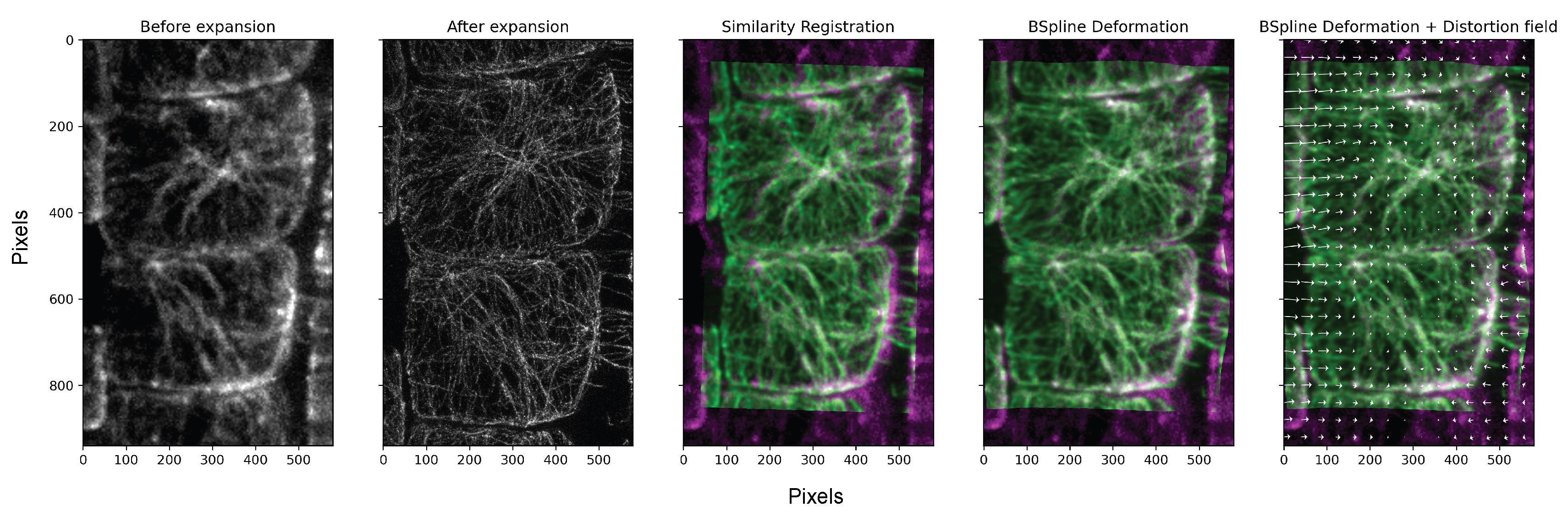
Figure 7. Image analysis results. Maximum-intensity projection images of Arabidopsis root cells immunostained with an anti-α-tubulin antibody. First, we selected and prepared similar images of the same sample before and after expansion, as shown in the greyscale image. The post-expansion image was linearly and then nonlinearly transformed to generate overlay images and distortion vector fields. The pre- and post-expansion images are displayed in magenta and green, respectively, in the overlay. These overlays and distortion vector fields are automatically generated using our scripts.
C. Reproducibility considerations
All analyses were performed using a fixed computational environment (Python 3.10.19; SimpleITK-SimpleElastix 2.0.0rc2.dev910; NumPy 2.2.6; SciPy 1.15.2; scikit-image 0.25.2; matplotlib 3.10.8; pandas 2.3.3). To ensure full reproducibility, the repository includes: (1) A human-readable environment specification (environment.yml); (2) an archived frozen environment (environment_frozen.yml) capturing the exact resolved dependency state; (3) a platform-specific explicit conda lock file (conda-lock-win64.txt); and (4) a pip dependency archive (requirements_pip_frozen.txt). Example datasets and references output files are provided to enable independent numerical validation of the analysis results. Automated regression tests are included to confirm installation integrity and numerical consistency.
Confocal laser scanning microscopy images before and after expansion were analyzed. The images are Arabidopsis root cells stained with an anti-α-tubulin primary antibody and a secondary antibody conjugated with Alexa Fluor 488. The pre- and post-expansion images are displayed in magenta and green, respectively, in the overlay (see Figure 7 and Figure S1). The post-expansion image shown in the overlay was after applying the Gaussian filter.
D. Visualization and interpretation
Root-ExM achieved a 4.3 ± 0.3 (mean ± SD)-fold expansion, while maintaining cellular morphology and structural integrity (Figure 8A–C). Comparing the pre- and post-expansion images, ExM substantially increases the signal-to-noise ratio and spatial resolution (Figure 8D). As expanded samples were optically clear, we were able to detect the signal over the whole root tissue, which corresponds to an axial distance of at least 400 μm, and image the immunostained microtubule at the most distant epidermal cells from the objective (Figure 8E). Microtubules often serve as biological nanorulers for super-resolution modalities because of their well-defined 25-nm diameter and their larger apparent size (typically 45–60 nm) when immunostained via conventional primary–secondary antibody labeling [13–15]. As in the original 4× ExM report, we observed the microtubule in detail. Using Alexa Fluor 488- and 594-conjugated secondary antibodies, we measured the apparent widths of cross-sectioned microtubules as 72.7 ± 8.3 nm and 85.6 ± 7.2 nm (mean ± SD), respectively (determined by the full width at half maximum of the Gaussian fit) (Figure 8F–H). These values are similar to the reported diameter of 82.4 nm in the original 4× ExM study [10]. Given that the apparent width results from the convolution of the point spread function (PSF ≈ effective resolution) with the actual microtubule dimensions (conservatively defined as 50 nm here), we estimate the lateral resolution to be ~60 and ~70 nm for green and red channels, respectively. These resolutions are consistent with the expansion factor–corrected theoretical diffraction limits of our microscope [a simple equation of Δr = λ/2NA·ExF; i.e., Δr = 58 nm for the wavelength (λ) of 500 nm as the green channel, numerical aperture (NA) of 1.0, and expansion factor (ExF) of 4.3; Δr = 70 nm for the λ of 600 nm as the red channel]. The correspondence between the practical and theoretical resolutions indicates that Root-ExM allows us to perform plant imaging in the optically ideal situation. Furthermore, the difference observed between Alexa Fluor 488- and 594-labeled microtubules highlights the wavelength-dependent resolution limit inherent in the conventional microscope.
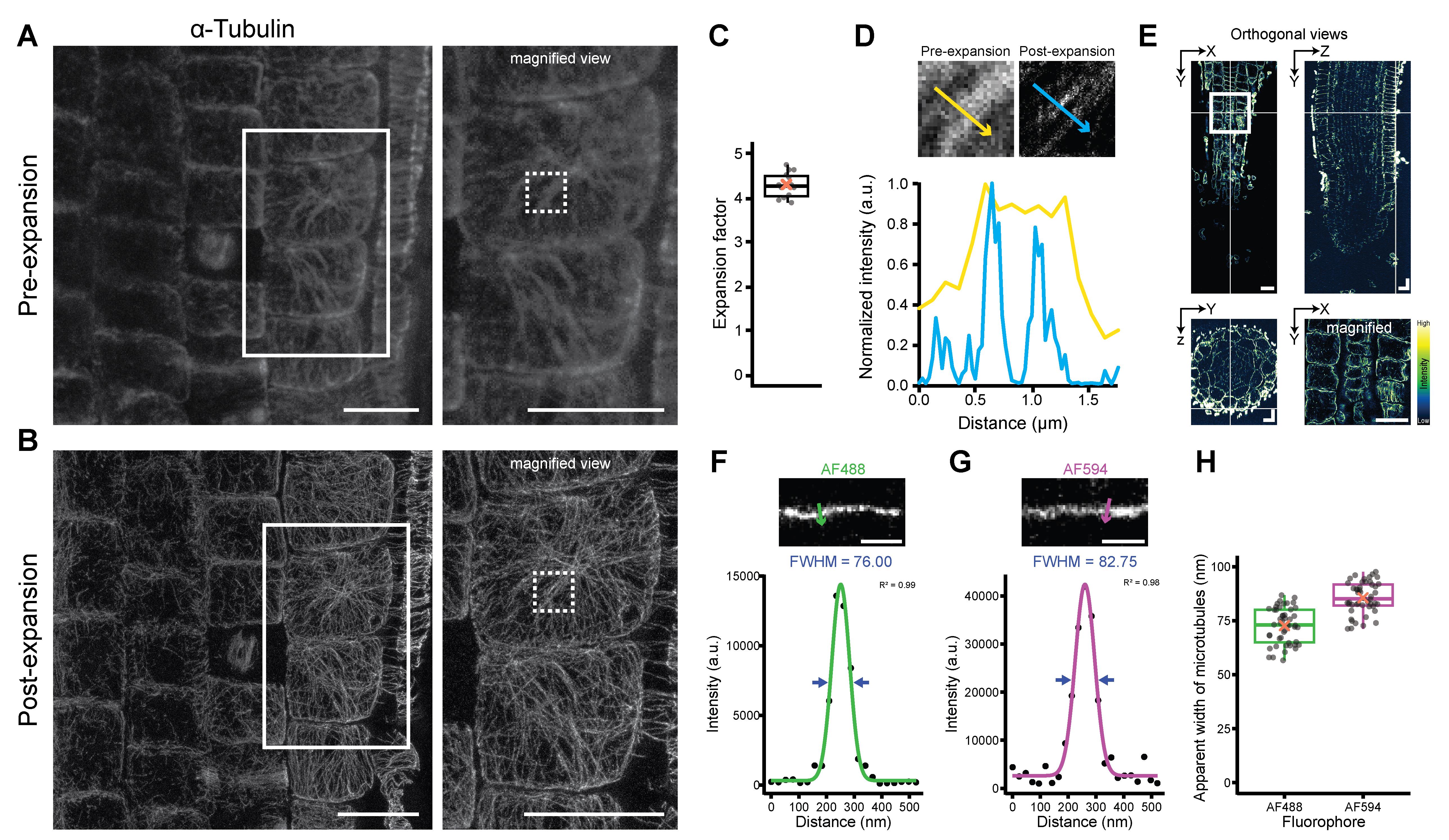
Figure 8. Super-resolution imaging of microtubules in Arabidopsis root cells by ROOT-ExM. (A, B) Confocal laser scanning microscopy images of a primary root stained with anti-α-tubulin primary antibody and a secondary antibody conjugated with Alexa Fluor 488 (AF488) before (A) and after expansion (B). The images are maximum-intensity projections of 6 optical sections spanning 4.7 μm (A, pre-expansion) and 26 optical sections spanning 17.5 μm (B, post-expansion) in terms of physical size. Expansion factor = 4.69. (C) Quantification of the expansion factor based on a comparison between the pre- and post-expansion fluorescence images (n = 16 roots from three independent experiments). (D) Comparison of fluorescence intensity profiles taken along the yellow and cyan lines. Fluorescence images are from dashed boxes in A and B but showing a single confocal plane. (E) Orthogonal view images of the primary root visualized with the anti-α-tubulin primary and AF488 secondary antibodies. The image was reconstructed from 150 optical sections spanning 447 μm in terms of physical size. Epidermal cells distal to the objective are presented in the magnified view image. Expansion factor = 4.12. (F, G) Exemplary quantification of microtubule diameter in ROOT-ExM. The anti-α-tubulin primary antibody was labeled with the secondary antibody conjugated with AF488 (F) or AF594 (G). The fluorescence intensity profiles along the arrows are plotted as dots. Solid lines indicate the Gaussian fit used to determine the full width at half maximum (FWHM). (H) Quantification of the apparent width of the microtubule labeled with AF488 or AF594 (n = 48 microtubules from three independent experiments). AF488 was excited with a 488 nm laser, and its fluorescence was detected at 499–561 nm. AF594 was excited with a 594 nm laser, and its fluorescence was detected at 597–686 nm. The pixel size was 120 nm (A, B, F, and G) or 350 nm (E). Scale bars = 10 μm (A, B, and E) or 1 μm (F and G) in the original biological scale.
Validation of protocol
This protocol has been used and validated in the following research articles:
• Grison et al. [12]. Root expansion microscopy: A robust method for super resolution imaging in Arabidopsis. The Plant Cell. https://doi.org/10.1093/plcell/koaf050
• Fougère et al. [16]. ER-to-Golgi trafficking through a dynamic intermediate cis-Golgi tubular network in Arabidopsis. Nature Cell Biology. https://doi.org/10.1038/s41556-025-01624-x
• Goldy et al. [17]. The actin cytoskeleton is required to maintain plant cell division orientation against cellular geometry. Science Advances. https://doi.org/10.1126/sciadv.aeb8498
General notes and troubleshooting
General notes
This protocol provides a robust and reproducible method for ExM of the Arabidopsis root cells in the meristematic, transition, and elongation zones. However, we observed that cells in the differentiation zone failed to expand, likely due to the deposition of secondary cell walls. This resulted in the fragmentation of differentiated root tissues within the expanded hydrogel. Accordingly, while ROOT-ExM appears suitable for tissues with characteristics similar to the Arabidopsis root tip, its direct application to tissues with greater mechanical rigidity may remain challenging.
While we take the microtubule as an example in this work, we successfully imaged various cellular compartments (Table 1).
Table 1. Cellular structures imaged by ROOT-ExM
| Structure | Reporter or probe | Ref. |
|---|---|---|
| Microtubule | Anti-α-tubulin antibody | [12,17] |
| Nucleus | DAPI or NHS ester | [12] |
| Nuclear envelope | Anti-SUN antibody | [12] |
| Endoplasmic reticulum (ER) | YFP-HDEL | [12] |
| ER–Golgi intermediate compartments (ERGIC) | Anti-MEMB antibody | [16] |
| Golgi medial cisterna | NAG1-GFP | [12,16] |
| Cell plate | Anti-KNOLLE antibody | [12] |
| Mitochondrion | NHS ester | [12] |
| Plasmodesma | NHS ester or anti-callose antibody | [12] |
| Cell wall | Calcofluor white Note: To obtain strong fluorescence signals, the second cell wall digestion (step 38) can be omitted or shortened | [12] |
Troubleshooting
| Problem | Possible cause | Solution |
| The gel does not polymerize | Oxygen may prevent proper acrylamide polymerization | Use a new aliquot of the monomer solution at each step (i.e., use one aliquot each for steps 29, 30, and 32). Avoid the contamination of tiny air bubbles in the gelation solution when placing the coverslip, and seal the gelation chamber tightly. |
| The monomer solution may be of insufficient quality | Use a new aliquot of the monomer solution at each step. If deterioration is suspected, make a new stock solution. | |
| TEMED or APS solution may be of insufficient quality | Make a new stock solution. | |
| Inappropriate addition of TEMED or APS. If not mixed instantly and thoroughly, polymerization could occur topically (e.g., at the surface only) | Mix thoroughly after each addition of 4-hydroxy-TEMPO, TEMED, and APS to the monomer solution. However, work quickly on ice to prevent the reaction from starting prematurely in the tube. | |
| The gel is not peeled off from the coverslip in the homogenization solution or ultrapure water | Strong association between the gel and the Poly-D-Lysine-coated glass surface | Trim away the gel from the coverslip by inserting a razor blade between the gel and coverslip after gelation completion (i.e., at step 33). |
| The expansion factor is significantly lower than expected (<3×) | Residual salts in the gel or solution inhibit expansion | Wash the gel at least 3–5 times in a large volume of fresh ultrapure water and increase the total incubation time. |
| Insufficient homogenization | Try prolonged proteinase K digestion (~24 h), perform an additional round of digestion by replacing the solution, or incubate the sample at 37 °C. | |
| Ruptures or severe distortions of the sample are observed after expansion | Insufficient homogenization | Try the above-mentioned proteinase K digestion. If deterioration is suspected, make a new stock solution. |
| Insufficient protein anchoring to the gel matrix | Incubate the sample in the Acryloyl-X, SE solution for 24 h rather than 20 h. If deterioration is suspected, make a new stock solution. | |
| Sodium acrylate, acrylamide, or methylenebisacrylamide may be of insufficient quality. | Make a new stock of the monomer solution. | |
| Structural integrity of cellular compartments (e.g., the cytoskeleton or endoplasmic reticulum) is not preserved or is poor | The fixation may not be adequate | Optimize the incubation time or try other fixatives. |
| The fluorescence is dim after expansion | Fluorescent molecules inevitably spread out during expansion, resulting in a decrease in signal per pixel | This normally occurs and is inevitable. Increase the laser power, exposure time, or detector gain. |
| Proteinase K digestion may be intense. Since proteinase K also digests fluorophore-conjugated antibodies or fluorescent proteins to some degree, the trade-off between the degree of homogenization and retention of fluorescence is unavoidable in the classical ExM | Optimize the digestion time. Alternatively, proExM with post-expansion labeling or proteinase-free homogenization approaches (e.g., autoclaving of the gel) can be attempted [11]. | |
| No fluorescence signal is detected | Antibody labeling of the protein of interest is not adequate | Acquire pre-expansion fluorescence images to check if the labeling works. If it does not work, optimize immunostaining protocols or change antibodies. |
| The protein of interest does not resist the fixation | Acquire pre-expansion fluorescence images to check if the protein of interest resists the fixation. If it does not, try other fixations. In case of using fluorescent marker lines, try switching to a different fluorescent protein version. | |
| The sample drifts during observation with the water objective | The gel does not adhere to the APTES-coated coverslip | This often happens. Remove the excess water surrounding the gel before placing it on the APTES-coated coverslip. Waiting to pour water for a few minutes after placing the gel helps it to settle into a stable position. |
| The sample cannot be located | The sample may be located on the opposite side (i.e., the side away from the objective) | Flip the gel and locate the sample again. |
Supplementary information
The following supporting information can be downloaded here:
1. Figure S1. Image analysis workflow
Acknowledgments
Imaging was performed at the Bordeaux Imaging Center (BIC), a part of the National Infrastructure France–BioImaging supported by the French National Research Agency (ANR-24-INBS-0005 FBI BIOGEN). We thank the staff of the BIC for providing support with protocol optimization and microscopy imaging. The study was supported by the grants ANR DIVCON (ANR-21-CE13-0016-01), ANR FATROOT (ANR-21-CE13-0019-02), ANR DivFUSE (ANR-22-CE92-0038-01), and HORIZON-MSCA-2024-PF-01 (no. 101207095).
Contributions of each author: Conceptualization, Y.S. and M.S.G.; Investigation, Y.S., G.M., F.D., and M.S.G.; Writing—Original Draft, Y.S., G.M., and M.S.G.; Writing—Review & Editing, M.F.-M, E.M.B., Y.B., and M.S.G.; Funding acquisition, Y.S., E.M.B., and Y.B.; Supervision, E.M.B., Y.B., and M.S.G.
The protocol described here is based on the previous work published in Grison et al. [12].
Competing interests
The authors declare no conflicts of interest.
References
- Hell, S. W. and Wichmann, J. (1994). Breaking the diffraction resolution limit by stimulated emission: stimulated-emission-depletion fluorescence microscopy. Opt Lett. 19(11): 780–782. https://doi.org/10.1364/ol.19.000780
- Betzig, E., Patterson, G. H., Sougrat, R., Lindwasser, O. W., Olenych, S., Bonifacino, J. S., Davidson, M. W., Lippincott-Schwartz, J. and Hess, H. F. (2006). Imaging intracellular fluorescent proteins at nanometer resolution. Science. 313(5793): 1642–1645. https://doi.org/10.1126/science.1127344
- Rust, M. J., Bates, M. and Zhuang, X. (2006). Sub-diffraction-limit imaging by stochastic optical reconstruction microscopy (STORM). Nat Methods. 3(10): 793–795. https://doi.org/10.1038/nmeth929
- Kumar, R. and Silva, L. (1973). Light ray tracing through a leaf cross section. Appl Opt. 12(12): 2950–2954. https://doi.org/10.1364/AO.12.002950
- Vogelmann, T. C., Bornman, J. F. and Yates, D. J. (1996). Focusing of light by leaf epidermal cells. Physiol Plant. 98(1): 43–56. https://doi.org/10.1111/j.1399-3054.1996.tb00674.x
- Carlsson, K. (1991). The influence of specimen refractive index, detector signal integration, and non‐uniform scan speed on the imaging properties in confocal microscopy. J Microsc. 163(2): 167–178. https://doi.org/10.1111/j.1365-2818.1991.tb03169.x
- Hell, S., Reiner, G., Cremer, C. and Stelzer, E. H. K. (1993). Aberrations in confocal fluorescence microscopy induced by mismatches in refractive index. J Microsc. 169(3): 391–405. https://doi.org/10.1111/j.1365-2818.1993.tb03315.x
- Diaspro, A., Federici, F. and Robello, M. (2002). Influence of refractive-index mismatch in high-resolution three-dimensional confocal microscopy. Appl Opt. 41(4): 685–690. https://doi.org/10.1364/ao.41.000685
- Pawley, J. (Ed.). (2006). Handbook of biological confocal microscopy (3rd ed.). PDF. New York, NY: Springer. https://doi.org/10.1007/978-0-387-45524-2
- Chen, F., Tillberg, P. W. and Boyden, E. S. (2015). Expansion microscopy. Science. 347(6221): 543–548. https://doi.org/10.1126/science.1260088
- Tillberg, P. W., Chen, F., Piatkevich, K. D., Zhao, Y., Yu, C.-C. J., English, B. P., Gao, L., Martorell, A., Suk, H.-J., Yoshida, F., et al. (2016). Protein-retention expansion microscopy of cells and tissues labeled using standard fluorescent proteins and antibodies. Nat Biotechnol. 34(9): 987–992. https://doi.org/10.1038/nbt.3625
- Grison, M. S., Maucort, G., Dumazel, A., Champelovier, D., Shimizu, Y., Boutté, Y., Fernández-Monreal, M. and Bayer, E. M. (2025). Root expansion microscopy: A robust method for super resolution imaging in Arabidopsis. Plant Cell. 37(4): koaf050. https://doi.org/10.1093/plcell/koaf050
- Ledbetter, M. C. and Porter, K. R. (1964). Morphology of microtubules of plant cell. Science. 144(3620): 872–874. https://doi.org/10.1126/science.144.3620.872
- Weber, K., Rathke, P. C. and Osborn, M. (1978). Cytoplasmic microtubular images in glutaraldehyde-fixed tissue culture cells by electron microscopy and by immunofluorescence microscopy. Proc Natl Acad Sci USA. 75(4): 1820–1824. https://doi.org/10.1073/pnas.75.4.1820
- Ries, J., Kaplan, C., Platonova, E., Eghlidi, H. and Ewers, H. (2012). A simple, versatile method for GFP-based super-resolution microscopy via nanobodies. Nat. Methods. 9(6): 582–584. https://doi.org/10.1038/nmeth.1991
- Fougère, L., Grison, M., Laquel, P., Montrazi, M., Cordelières, F., Fernández-Monreal, M., Poujol, C., Uemura, T., Nakano, A., Ito, Y., et al. (2025). ER-to-Golgi trafficking through a dynamic intermediate cis-Golgi tubular network in Arabidopsis. Nat Cell Biol. 27(3): 424–437. https://doi.org/10.1038/s41556-025-01624-x
- Goldy, C., Moulin, S., Shimizu, Y., Cerutti, G., Bayle, V., Grison, M., Jaillais, Y., Bouchez, D., Boutté, Y., Pastuglia, M., et al. (2026). The actin cytoskeleton is required to maintain plant cell division orientation against cellular geometry. Sci Adv. 12(8): eaeb8498. https://doi.org/10.1126/sciadv.aeb8498
- Chozinski, T. J., Halpern, A. R., Okawa, H., Kim, H. J., Tremel, G. J., Wong, R. O. and Vaughan, J. C. (2016). Expansion microscopy with conventional antibodies and fluorescent proteins. Nat Methods. 13(6): 485–488. https://doi.org/10.1038/nmeth.3833
Article Information
Publication history
Received: Mar 10, 2026
Accepted: Apr 27, 2026
Available online: May 13, 2026
Published: Jun 5, 2026
Copyright
© 2026 The Author(s); This is an open access article under the CC BY-NC license (https://creativecommons.org/licenses/by-nc/4.0/).
How to cite
Shimizu, Y., Maucort, G., Fernández-Monreal, M., Dumas, F., Bayer, E., Boutté, Y. and Grison, M. (2026). ROOT-ExM: Super-Resolution Imaging of Proteins in Arabidopsis Roots by Expansion Microscopy. Bio-protocol 16(11): e5707. DOI: 10.21769/BioProtoc.5707.

 Download Citation in RIS Format
Category
Plant Science > Plant cell biology > Cell imaging
Cell Biology > Cell imaging > Super resolution imaging
Cell Biology > Tissue analysis > Tissue imaging
Do you have any questions about this protocol?
Post your question to gather feedback from the community. We will also invite the authors of this article to respond.
 Post a Question


