


- Protocols

- Articles and Issues
- For Authors
- About
- Become a Reviewer


Accessible STORM Imaging: An Optimized Workflow for Conventional Widefield Epifluorescence/TIRF Setups

(*contributed equally to this work) Published: Vol 16, Iss 8, Apr 20, 2026 DOI: 10.21769/BioProtoc.5672 Views: 697
Reviewed by: Elena A. OstrakhovitchKM Rifat FaysalAnonymous reviewer(s)
 PDF
PDF  Ask a question
Advertisement



Protocol Collections
Comprehensive collections of detailed, peer-reviewed protocols focusing on specific topics




Related protocols
Abstract
Stochastic optical reconstruction microscopy (STORM) is a single-molecule localization microscopy technique that enables visualization of cellular structures beyond the diffraction limit. This approach has revealed previously inaccessible ultrastructural details in a wide range of cellular components, including the actin cytoskeleton, clathrin-coated pits, mitochondria, and bacterial nucleoid-associated proteins. STORM relies on the sequential emission of single photons from photosensitive fluorophores, which are precisely localized before entering a dark state or undergoing photobleaching. By activating fluorophores individually and fitting their point spread functions (PSFs), the center of mass can be calculated with a localization precision of up to ~20 nm. The parallel detection of thousands of single-molecule events, each assigned to distinct spatial coordinates, enables the reconstruction of a high-resolution image. Here, we describe a simple and efficient STORM workflow—including sample preparation, image acquisition, and quality control measurements—that we used to visualize various subcellular structures, such as mitochondria, microtubules, and lysosomes labeled with the commonly employed cyanine dye Alexa Fluor 647, as well as the actin cytoskeleton stained with Alexa Fluor 488–conjugated phalloidin. Image acquisition was performed using a conventional epifluorescence/total internal reflection (TIRF) microscope adapted for STORM imaging. Key adaptations included the use of a 160×/1.43 NA oil-immersion objective and a high-power mode, which concentrates the laser beam onto a small region of the sample, ensuring sufficient light intensity to drive fluorophores into the dark state. In addition, implementing a 1.6× magnification lens and a 4×4 binning camera mode allowed us to achieve a 100-nm pixel size optimal for reliable molecule detection. We believe that this protocol will be highly valuable to the microscopy community, as it lowers technical barriers to performing STORM on widely available microscopy platforms, thereby facilitating broader implementation of this powerful super-resolution technique.
Key features
• Optimized immunofluorescence, including multiple washing steps using 0.1% Tween-20 and a secondary antibody fixation step for single and dual-color STORM.
• Imaging acquisition performed with a conventional epifluorescence/TIRF microscope adapted for STORM imaging.
• Use of a 160×/1.43 NA oil-immersion objective and a high-power mode that concentrates the laser beam onto a small region of the sample.
• Implementation of a 1.6× magnification lens and 4 × 4 camera binning to achieve 100 nm pixel size.
Keywords: STORM SMLM
Lysosomes
Microtubules
Mitochondria
Actin
TIRF
Uncertainty
FWHM
SMLM
Lysosomes
Microtubules
Mitochondria
Actin
TIRF
Uncertainty
FWHM
Graphical overview
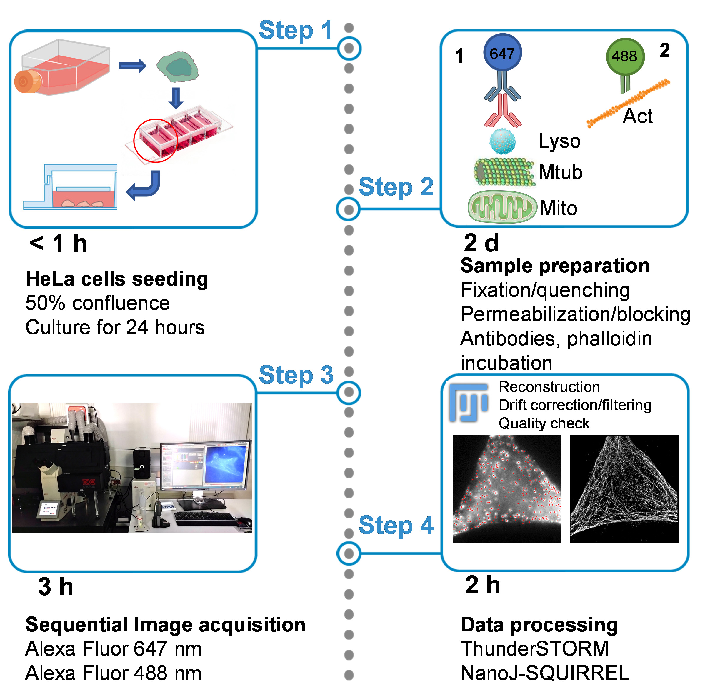
Step-by-step workflow for stochastic optical reconstruction microscopy (STORM) imaging. The graphical summary outlines all the critical steps of the workflow and highlights the time required for each stage. (Step 1) HeLa cells are seeded in dedicated four-well imaging chambers and cultured for 24 h to allow cell adhesion. (Step 2, left) Cells are then fixed and quenched, an essential step to decrease auto-fluorescence, followed by permeabilization and blocking, a crucial step to avoid unspecific antibody binding. Different samples are prepared using distinct primary antibodies to visualize different cellular structures, including lysosomes (Lyso) and microtubules (Mtub) for single-color STORM, as well as mitochondria (Mito) for dual-color STORM. We used the corresponding secondary antibody, conjugated with Alexa Fluor 647, matched to the host species of the primary antibody. (Step 2, right) For mitochondria-labeled dual-color STORM samples, filamentous actin was additionally stained using phalloidin-Alexa Fluor 488. (Step 3) Imaging acquisition is performed in STORM imaging buffer using a widefield/total internal reflection (TIRF) system. Sequential acquisition is required for dual-color samples, with Alexa Fluor 647 imaged first, followed by Alexa Fluor 488. (Step 4) The final step involves data processing with the ThunderSTORM plugin, which consists of single-molecule localization, drift correction, and filtering to generate the final STORM reconstructed image. The quality check of the resulting images is performed with the NanoJ-SQUIRREL plugin.
Background
The discovery of super-resolution imaging methods has enabled optical microscopy to overcome the conventional light diffraction limit, defined by Ernst Karl Abbe in 1873. These methods have completely revolutionized the field of optical fluorescence microscopy, tremendously enhancing its resolution power [1]. Single-molecule localization microscopy (SMLM) techniques rely on the precise determination of fluorophore positions, with subpixel accuracy, based on the emission from a small molecule subset, which can be distinguished from nearby fluorophores in the dark (non-emitting) state, thus allowing the reconstruction of a high-resolution image [2,3]. The strategy applied to achieve the fluorophore on/off state switching is specific to each SMLM technique, which mainly includes photo-activated localization microscopy (PALM) and stochastic optical reconstruction microscopy (STORM). Briefly, PALM can also be applied to live-cell imaging and relies on the use of photoactivatable/switchable proteins, which can be activated with near-UV/violet light (typically ~405 nm) or photo-converted from a shorter to a longer wavelength form. The detection of emission by single molecules is achieved using low-intensity activation or switching laser cycles, which turn on or convert only a subset of fluorophores at a time, until they are photobleached [4]. In contrast, STORM exploits organic fluorophores such as Alexa Fluor–conjugated antibodies (e.g., Alexa Fluor 647), which undergo reversible photo switching in suitable imaging buffers; therefore, it is suitable for fixed sample imaging [5].
STORM is a single-molecule high-resolution microscopy technique that allows the visualization of unresolved details of many cellular structures, including clathrin-coated pits, mitochondria, synaptic structures, and neuronal spectrin, which forms, with actin and associated proteins, a periodic structure in neurons [6–9]. In addition, the technique relies on fluorophores blinking, defined as the stochastic switching of a photosensitive molecule between fluorescent (on) and non-fluorescent (off) states, enabling the precise localization of individual emitters, before they enter a long-lived dark state or become photobleached. The localization coordinates of many individuals emitting fluorophores, each associated with respective spatial coordinates, allow the reconstruction of a high-resolution image [10]. The implementation of advanced imaging methods for broader laboratory use highlights the need for rigorous validation strategies and quantitative performance metrics supporting protocol optimization and cross-platform reproducibility in quantitative imaging workflows [11].
The current protocol describes a complete workflow, including sample preparation, image acquisition, data processing, and quality assessment to obtain high-quality single and dual-color STORM images of different cellular structures such as tubulin, lysosomes, mitochondria, and the actin cytoskeleton. Here, we employed commercially available primary antibodies and secondary antibodies conjugated to Alexa Fluor 647 switchable fluorophores, which show excellent blinking properties and represent the most widely used dyes for STORM imaging. In addition, for dual-color experiments, the actin cytoskeleton was labeled using a phalloidin-Alexa Fluor 488, which allows high-quality reconstruction of the cytoskeleton, although its blinking properties are lower than those of the Alexa Fluor 647 counterpart [12]. For imaging, an oxygen-scavenging imaging buffer, which maintains a reducing chemical environment ideal for the dye photo conversion, is used. The choice to perform dual-color STORM using an Alexa Fluor 647/Alexa Fluor 488 combination was dictated by the excitation–emission filter of our system, as well as the compatibility of the two dyes with the imaging buffer, which needs to be adjusted and optimized according to the chemical properties of the fluorophores.
Despite the growing interest in super-resolution microscopy, the implementation of STORM often requires specialized instrumentation and technical expertise that may not be readily available in many laboratories. This protocol addresses this gap by providing a workflow that enables STORM imaging using widely available microscopy platforms with minimal technical modifications. By lowering the technical barriers to SMLM implementation, this approach aims to facilitate broader adoption of super-resolution imaging across research laboratories. Such accessibility could benefit diverse applications, including studies of cellular architecture, mechanotransduction, and tissue organization, where nanoscale imaging can provide insights into biological processes such as osteocyte responses to mechanical stress [13]. STORM imaging requires customized microscopes or commercially available systems, which are specifically designed for SMLM experiments, including the ONI imager (www.oni.bio.com) or the Abbelight platform (www.abbelight.com). This represents a limitation to the spreading of this powerful microscopy technique. In order to overcome this limitation, we designed this protocol where image acquisition is performed on a conventional epifluorescence/total internal reflection (TIRF) microscope, commonly available in many laboratories or imaging facilities, adapted for STORM imaging. Crucial adaptations include the use of a 160×/1.43 NA oil-immersion objective and a high-power mode that concentrates the laser beam onto a small region of the sample, ensuring sufficient intensity to drive fluorophores into the dark state. This allows us to overcome the limitation of the low laser power compared to the system designed for STORM, which shows high-power laser beams. Indeed, power ranges (at samples) for 638 and 488 nm laser lines are on the order of 250 mW for ONI or 40–500 mW for Abbelight microscopes, compared to 25–30 mW for our system used here. In addition, implementing a 1.6× magnification lens and a 4×4 binning camera mode allowed us to achieve a 100-nm effective pixel size optimal for reliable molecule detection. Moreover, the use of TIRF microscopy, which allows regulation of laser penetration depth within the sample [14], helps with background removal, optimizing the molecule localization during image analysis. Image reconstruction and post-processing drift correction, as well as the evaluation of the quality of molecule localization, were performed using the ThunderSTORM open-source Fiji plugin tool [15]. The quality of STORM reconstructed images was assessed using the NanoJ-SQUIRREL open-source Fiji plugin [16], comparing the corresponding TIRF image.
These developments aim to improve the accessibility of STORM imaging and reduce technical barriers to its implementation, facilitating broader adoption of super-resolution microscopy in standard laboratory environments. Such efforts align with recent methodological advances emphasizing translational robustness and standardized experimental workflows to ensure reproducibility across research settings [17]. We believe that this protocol will be particularly valuable to the microscopy community, especially for beginner STORM users, as it can be implemented on widely available microscopy platforms already available in many laboratories or imaging facilities. With minor technical adjustments, these platforms can be adapted for SMLM imaging, avoiding substantial financial investments.
Materials and reagents
Biological materials
1. HeLa cell line (American Type Culture Collection, catalog number: CCL2)
Reagents
1. Dulbecco’s phosphate buffered saline (PBS) (Merck Life Science, catalog number: D8537)
2. Dulbecco’s modified Eagle medium (DMEM) high glucose (Biowest, catalog number: L0101-500)
3. Fetal bovine serum (FBS) (Sigma, catalog number: F-7524)
4. L-Glutamine 100 mM (Biowest, catalog number: X0550)
5. Sodium pyruvate 100 mM (Biowest, catalog number: L0642)
6. Ethylenediaminetetraacetic acid (EDTA) Tritiplex III (Merck, catalog number: 1.08418)
7. Sodium hydroxide (NaOH) (Merck, catalog number: 1370311002)
8. Paraformaldehyde (PFA) 16% w/v aqueous solution, methanol-free (Thermo Fisher Scientific, catalog number: 043368.9M)
9. Glutaraldehyde solution, 50 wt% in H2O (Sigma, catalog number: 340855)
10. Triton X-100 (Sigma, catalog number: T9284)
11. Sodium borohydride (Merck, catalog number: 452882)
12. Tween 20 (Sigma, catalog number: P6585)
13. D-(+)-glucose (Merck, catalog number: 1.08337.0250)
14. Cysteamine (Sigma, catalog number: 30070); store at 4 °C
15. Glucose oxidase from Aspergillus niger (Merck, catalog number: G2133); store at -20 °C
16. Catalase from bovine liver (Merck, catalog number: C40); store at -20 °C
17. Mouse anti-LAMP2 (H4B4) primary antibody (Santa Cruz, catalog number: SC-18822)
18. Goat anti-mouse Alexa Fluor 647 (Thermo Fisher Scientific, catalog number: A21236); store at -20 °C
19. Mouse anti-tubulin primary antibody (Sigma, catalog number: T5168)
20. Rabbit anti-TOMM22 primary antibody (Sigma, catalog number: HPA003037)
21. Goat anti-rabbit Alexa Fluor 647 (Thermo Fisher Scientific, catalog number: A21245)
22. Phalloidin-Alexa Fluor 488 (Thermo Fisher Scientific, catalog number: A12379); store at -20 °C
Solutions
1. HeLa cell culture medium (see Recipes)
2. EDTA 0.5 M stock (see Recipes)
3. PBS-EDTA (see Recipes)
4. Fixation solution (see Recipes)
5. Quenching solution (see Recipes)
6. Permeabilization buffer (see Recipes)
7. Blocking/antibody buffer (see Recipes)
8. Washing buffer (see Recipes)
9. Antibody fixation solution (see Recipes)
10. Cysteamine (see Recipes)
11. D-glucose 25% (see Recipes)
12. Glucose oxidase (see Recipes)
13. Catalase (see Recipes)
14. Imaging buffer (see Recipes)
Recipes
1. HeLa cell culture medium
| Reagent | Final concentration | Quantity or volume |
|---|---|---|
| DMEM (4.5 g/L D-glucose) | n/a | 440 mL |
| L-Glutamine | 1% (v/v) | 5 mL |
| Sodium pyruvate | 1% (v/v) | 5 mL |
| FBS | 10% (v/v) | 50 mL |
| Total | n/a | 500 mL |
2. EDTA 0.5 M stock
| Reagent | Final concentration | Quantity or volume |
|---|---|---|
| EDTA | 0.5 M | 9.3 g |
| MilliQ water | n/a | Up to 50 mL |
| Total | n/a | 50 mL |
Adjust pH to 7.8 using sodium hydroxide (NaOH). Filter solution with 0.22 μm filter.
3. PBS-EDTA
| Reagent | Final concentration | Quantity or volume |
|---|---|---|
| EDTA (0.5 M stock) | 10 mM | 1 mL |
| 1× PBS | n/a | 49 mL |
| Total | n/a | 50 mL |
4. Fixation solution
| Reagent | Final concentration | Quantity or volume |
|---|---|---|
| PFA 16% | 3% (v/v) | 0.544 mL |
| Glutaraldehyde (50 wt%) | 0.1% (v/v) | 0.0058 mL |
| 1× PBS | n/a | 2.35 mL |
| Total | n/a | 2.9 mL |
Critical: Prepare the fixation solution fresh before use. Store reagents at room temperature until their expiration. Opened paraformaldehyde stock ampoules can be stored at room temperature for up to 1 month.
Caution: Paraformaldehyde and glutaraldehyde are toxic and hazardous; wear a lab coat, gloves, and safety goggles. Perform all steps in a chemical safety hood and dispose of waste according to local regulations.
5. Quenching solution
| Reagent | Final concentration | Quantity or volume |
|---|---|---|
| Sodium borohydride | 0.1% (w/v) | 10 mg |
| 1× PBS | n/a | 10 mL |
| Total | n/a | 10 mL |
Critical: Prepare fresh before use. Store sodium borohydride at room temperature until expiring date.
Caution: Sodium borohydride is toxic and hazardous, and releases flammable hydrogen gas upon dissolution. Handle in a chemical safety hood and dispose of waste according to local regulations.
6. Permeabilization solution
| Reagent | Final concentration | Quantity or volume |
|---|---|---|
| Triton X-100 | 0.1% (v/v) | 0.003 mL |
| 1× PBS | n/a | 2.997 mL |
| Total | n/a | 3 mL |
7. Blocking/antibody solution
| Reagent | Final concentration | Quantity or volume |
|---|---|---|
| FBS | 10% (v/v) | 0.3 mL |
| 1× PBS | n/a | 2.7 mL |
| Total | n/a | 3 mL |
8. Washing buffer
| Reagent | Final concentration | Quantity or volume |
|---|---|---|
| Tween 20 | 0.1% (v/v) | 0.05 mL |
| 1× PBS | n/a | Up to 50 mL |
| Total | n/a | 50 mL |
9. Antibody fixation solution
| Reagent | Final concentration | Quantity or volume |
|---|---|---|
| PFA 16% | 1% (v/v) | 0.188 mL |
| 1× PBS | n/a | 2.812 mL |
| Total | n/a | 3 mL |
10. Cysteamine
| Reagent | Final concentration | Quantity or volume |
|---|---|---|
| Cysteamine | 1 M | 0.775 mg |
| MilliQ water | n/a | Up to 10 mL |
| Total | n/a | 10 mL |
Prepare single-use aliquots to avoid freeze-thaw cycles and store at -20 °C for up to 6 months.
11. D-glucose 25%
| Reagent | Final concentration | Quantity or volume |
|---|---|---|
| D-(+)-glucose | 25% (w/v) | 2.5 g |
| MilliQ water | n/a | Up to 10 mL |
| Total | n/a | 10 mL |
Prepare single-use aliquots to avoid freeze-thaw cycles and store at -20 °C for up to 6 months.
12. Glucose oxidase
| Reagent | Final concentration | Quantity or volume |
|---|---|---|
| Glucose oxidase | 2 mg/mL | 2 mg |
| 1× PBS | n/a | 1 mL |
| Total | n/a | 1 mL |
Prepare single-use aliquots to avoid freeze-thaw cycles and store at -20 °C for up to 6 months.
13. Catalase
| Reagent | Final concentration | Quantity or volume |
|---|---|---|
| Catalase | 2 mg/mL | 20 mg |
| 1× PBS | n/a | 10 mL |
| Total | n/a | 10 mL |
Prepare single-use aliquots to avoid freeze-thaw cycles and store at -20 °C for up to 6 months.
14. Imaging buffer
| Reagent | Final concentration | Quantity or volume |
|---|---|---|
| Cysteamine | 100 mM | 0.1 mL |
| D-glucose 25% | 5% | 0.2 mL |
| Glucose oxidase | 0.5 mg/mL | 0.25 mL |
| Catalase | 0.04 mg/mL | 0.02 mL |
| 1× PBS | n/a | 0.430 mL |
| Total | n/a | 1 mL |
Imaging buffer remains stable for up to 3 h during imaging at room temperature when protected from light. For longer imaging sessions, replace with fresh buffer.
Laboratory supplies
1. μ-slide 4-well Ph+ glass bottom # 1.5 (Ibidi, catalog number: 80447)
Equipment
1. Biological culture cabinet (Heraeus Instruments, model: LaminAir HB2436)
2. Cell culture incubator (Binder, model: CB150)
3. Microcentrifuge (Hettich Zentrifugen, model: Universal 320R)
4. Widefield microscope equipped with a total internal reflection fluorescence (TIRF) microscopy module, a high-power mode lens, and a 1.6× magnification lens (Leica, model: DMi8s)
5. Orca Flash 4.0 sCMOS camera (Hamamatsu, model: C13440)
6. HC PL APO 160×/1.43 NA oil immersion objective (Leica, catalog number: 11888434)
7. GFP filter set (Leica, catalog number: B0FF001E019016E0)
8. QUA-T filter set (Leica, catalog number: 623D011E019016E0)
Software and datasets
1. Fiji (www.imageJ.net/software/fiji), open-source software
2. Leica Application Suite (LAS X) (Leica, version 3.7.6.25997)
3. ThunderSTORM (open-source Fiji plugin)
4. NanoJ-SQUIRREL (open-source Fiji plugin)
5. GraphPad Prism (Dotmatics, version: 10)
Note: The ThunderSTORM analysis parameters, including localization thresholds and filtering criteria, were optimized individually for each cellular structure. These optimized parameters were then applied consistently across all datasets corresponding to the same structure to ensure reproducible image reconstruction. For NanoJ-SQUIRREL analysis, default parameters were used.
Procedure
A. Cell culture
1. Culture HeLa cells in a tissue culture flask using the DMEM medium under standard culture conditions [5% (v/v) CO2-enriched air at 37 °C].
2. For optimal culture maintenance, grow cells to ~80% confluency and detach them using PBS-EDTA.
3. Evaluate cell growth qualitatively by assessing culture surface coverage.
B. Cell seeding in a μ-slide 4-well Ph+ glass bottom # 1.5
Note: This step describes the cell preparation procedure and seeding in a multi-well dish, suitable for TIRF microscopy as well as single-molecule localization techniques, to allow adhesion and spreading. These slides were chosen because they allow long-term sample storage and extended imaging sessions.
1. Wash cells and detach them from a tissue culture flask.
a. Remove culture medium by gentle aspiration.
b. Wash cells once with sterile 1× PBS.
c. Add 3 mL of 10 mM PBS-EDTA solution.
d. Incubate cells at 37 °C for 3 min.
e. Check under the microscope if the cells have completely detached from the plate.
f. Add 4 mL of complete medium to stop the EDTA reaction and rinse the flask.
g. Collect the cell suspension in a sterile tube.
2. Determine cell concentration using a Neubauer counting chamber.
a. Gently mix cells with a sterile 5 mL culture pipette.
b. Load 10 μL of cell suspension and fill the counting chamber.
c. Count all viable cells included in the grid composed of four large square regions.
d. Calculate the average count and multiply by 10,000 to obtain the cell concentration (cells/mL).
e. Transfer the appropriate volume corresponding to 50,000 cells/well into a sterile 1.5 mL microcentrifuge tube.
3. Cell centrifugation and seeding:
a. Centrifuge the cell suspension at 114 rcf for 5 min at RT.
b. Remove the PBS-EDTA solution by aspiration.
c. Resuspend cells in the appropriate volume (700 μL/well) with fresh culture medium.
d. Seed cells into the μ-slide 4-well Ph+ glass bottom by filling the well completely using a P1000 pipette and cover with the lid.
e. Culture cells for 24 h under standard conditions.
Critical: Avoid air bubbles during mixing and especially during the seeding step.
C. Sample fixation, quenching, and permeabilization
Note: A combination of paraformaldehyde and low concentrations of glutaraldehyde was selected to enhance ultrastructural preservation and minimize molecular mobility during imaging. This fixation strategy improves structural stability while maintaining antigen accessibility, which is critical for accurate single-molecule localization in STORM microscopy. It is important to emphasize that controlled fixation and stepwise optimization in high-resolution imaging workflows are crucial for reliable results [11].
1. Cell fixation, sample quenching, and permeabilization
a. Gently remove 700 μL/well of culture medium using a P1000 pipette.
b. Add 700 μL/well of fixation solution.
c. Incubate for 20 min at room temperature.
d. Wash three times with 1× PBS (700 μL/well).
e. Add 700 μL/well of quenching solution.
f. Incubate for 5 min at room temperature.
g. Wash three times with 1× PBS (700 μL/well).
h. Add 700 μL/well of 0.1% Triton X-100 solution.
Critical: Prepare fresh before use. Store Triton X-100 stock at room temperature until expiration.
i. Incubate for 10 min at room temperature.
j. Wash three times with 1× PBS (700 μL/well).
Pause point: The protocol can be stopped after quenching or permeabilization. Store samples at 4 °C for up to 24 h.
D. Protein blocking and immunofluorescence
Note: Protein blocking is essential to prevent nonspecific primary antibody binding.
1. Remove PBS and replace with 700 μL/well of blocking solution.
Critical: The blocking solution must be freshly prepared.
2. Incubate for 1 h at room temperature.
3. Perform immunofluorescence staining. For the single-color STORM protocol, mouse anti-LAMP2 or mouse anti-tubulin primary antibody was used to label lysosomes or microtubules, respectively. For dual-color STORM, rabbit anti-TOMM22 primary antibody was used for mitochondrial labeling.
a. Replace blocking solution with 700 μL/well of the corresponding primary antibody, diluted (1:200) in blocking solution.
b. Incubate overnight at 4 °C.
c. Wash six times with the washing solution (700 μL/well, 5 min per wash).
Critical: Wash steps with PBS-Tween (PBS-T) after antibody incubations are essential to eliminate background fluorescence due to nonspecific antibody binding. This is a crucial step in STORM because, due to the high resolution reached, antibodies on glass are observed.
d. Add 700 μL/well of the goat anti-mouse Alexa Fluor 647 secondary antibody (1: 250) prepared in blocking solution.
e. Incubate for 1.5 h at room temperature in the dark.
f. Wash six times with washing solution (700 μL/well, 5 min per wash).
Critical: Wash steps with PBS Tween (PBS-T) after antibody incubations are essential to eliminate background fluorescence due to nonspecific antibody binding. This is a crucial step in STORM because, due to the high resolution reached, antibodies on glass are observed.
4. Fix antibodies with antibody fixation solution.
a. Replace PBS with 700 μL/well of antibody fixation solution.
b. Incubate for 15 min at room temperature in the dark.
c. Wash three times with 1× PBS (700 μL/well).
Pause point: Samples can be stored at 4 °C after this step.
5. Replace PBS with freshly prepared STORM imaging buffer.
Note: Imaging buffer must be freshly prepared. All components must be aliquoted and stored at -20 °C.
E. Filamentous actin staining with phalloidin-Alexa Fluor 488
Note: This step is performed only for dual-color STORM experiments. Here, we combine phalloidin staining in samples in which mitochondria have been labeled.
1. Incubate samples with phalloidin Alexa Fluor 488 diluted in PBS.
a. Add 700 μL/well of phalloidin Alexa Fluor 488 solution.
b. Incubate for 1 h at room temperature in the dark.
c. Remove staining solution and replace with PBS.
Critical: Do not wash after phalloidin staining to avoid excessive loss of dye molecules required for efficient signal replenishment during imaging.
F. Image acquisition
This section describes microscope settings and acquisition parameters for detecting blinking events in the far red and green channels using Alexa Fluor 647 and Alexa Fluor 488 cyanine dyes, respectively.
Figure 1 shows tubulin labeled with a standard Alexa Fluor 647-conjugated secondary antibody. Cells are focused and positioned using epifluorescence-TIRF mode, with the orange square highlighting the region of interest analyzed by STORM (Figure 1A). Figure 1B illustrates bleaching, allowing to reach the dark state of the molecules and subsequent blinking events (yellow dots) corresponding to single molecules emitting independently during acquisition cycles (Figure 1B). Reconstructed and processed STORM image of microtubules (Figure 1C) highlights the substantial resolution improvement compared to conventional TIRF imaging.
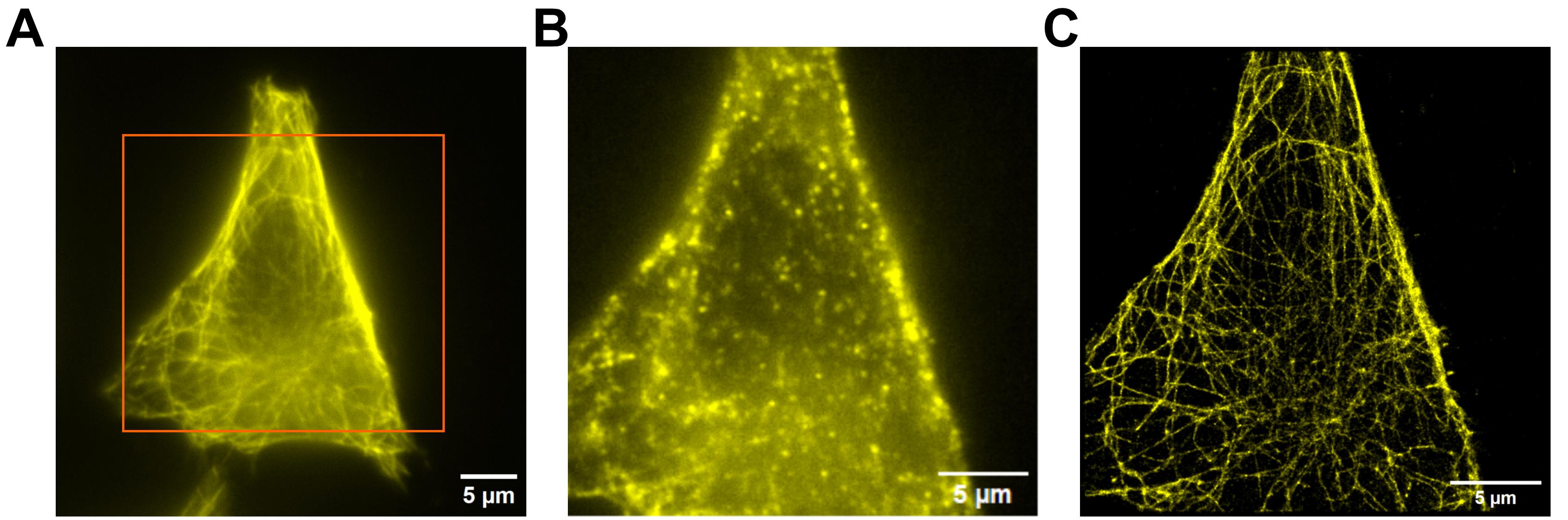
Figure 1. Representative example of tubulin labeled with an Alexa Fluor 647-conjugated secondary antibody showing fluorophore blinking and stochastic optical reconstruction microscopy (STORM) reconstruction. (A) Cells focused using standard epifluorescence–total internal reflection (TIRF) mode. The orange square region represents the area analyzed by STORM. (B) Bleaching allows reaching the dark state of molecules; blinking events (yellow dots) represent single molecules emitting separately during imaging cycles. (C) Resulting reconstructed and processed STORM image of microtubules. Scale bars, 5 μm.
The details of the microscope imaging settings are summarized in Figure 2.
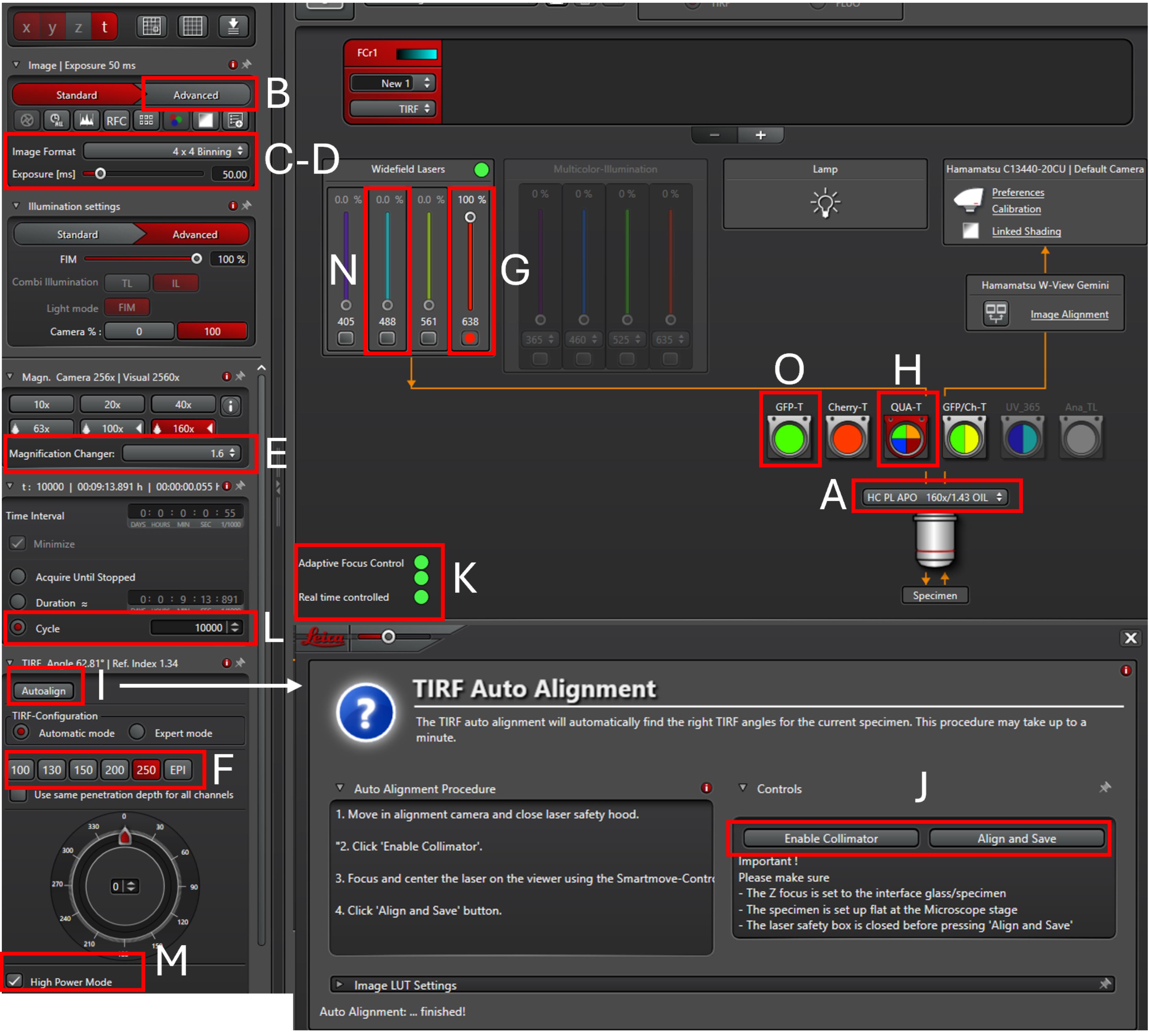
Figure 2. Summary of the microscope imaging settings. Crucial parameters are highlighted and summarized below: (A) HC PL APO 160× oil immersion objective. (B) Advanced camera settings (streaming mode). (C) Exposure time. (D) Camera 4 × 4 binning. (E) 1.6× magnification lens. (F) Total internal reflection (TIRF) penetration depth (between 150 and 250 nm). (G, H) 638 nm laser line and QUA-t emission filter for far-red TIRF imaging, corresponding to Alexa Fluor 647. (I) TIRF auto-alignment tool activation. (J) TIRF auto-alignment tool window. (K) Adaptive focus control (AFC). (L) Number of acquisition cycles. (M) High power mode. (N, O) 488 nm laser line and GFP emission filter for GFP-TIRF imaging, corresponding to Phalloidin Alexa Fluor 488.
1. Load the sample onto the microscope stage and adjust imaging parameters using Leica LAS X software.
a. Add one drop of immersion oil to the objective.
b. Place the slide into the stage microscope adapter.
c. Secure the slide using magnetic blockers.
d. Select HC PL APO 160×/1.43 NA oil immersion objective.
e. Enable advanced camera settings from the LAS X configuration option.
f. Activate camera streaming mode from the acquisition section of the camera settings.
g. Define exposure time to 50 ms.
h. Select 4 × 4 binning mode.
i. Select the 1.6× magnification lens.
2. Focus cells, align TIRF system, and adjust the critical TIRF penetration depth as well as the angle.
a. Select the far-red (Alexa Fluor 647)-TIRF channel (laser 638 nm and corresponding QUA-T filter are selected automatically).
b. Focus cells with very low laser power, selecting the epifluorescence EPI mode.
c. Perform laser alignment using the auto alignment function by activating the enable collimator option. Once this is done, activate the Align tool. Once the process is done correctly, close the auto-alignment window.
Note: This step is performed once immediately before starting image acquisition.
Critical: Proper laser alignment is essential for correct TIRF performance.
d. Adjust focus and optimize TIRF depth penetration and angle by qualitative inspection until the image appears clean, structures are well defined, and background fluorescence is minimized.
Critical: TIRF depth penetration adjustment depends on the structure being analyzed. Usually, between 150 and 250 nm works fine.
3. Capture a single image of the cell in standard TIRF mode to serve as a reference for quality assessment. Then, start the imaging series acquisition to record the blinking for STORM.
Note: This is required to have a comparison with the STORM image as well as for the quality assessment step.
a. Activate the Adaptive Focus Control (AFC) option.
Critical: It is essential to activate the focus control system to maintain focus during acquisition. AFC function is specific to Leica microscopes; however, the corresponding functionality can be differentially named in other imaging systems (i.e., Zero Drift Compensation for Olympus or Definite Focus for Zeiss).
b. Set the number of acquisition cycles to 10,000.
c. Set laser power to 100% until complete bleaching is achieved.
Note: The optimal laser power range is in the order of 7.5–8 μW for TIRF with 250 nm penetration depth.
d. Activate High Power Mode function to concentrate the laser beam on the sample and start the image series acquisition to record fluorophore blinking events.
e. During acquisition, decrease laser power to 70% to achieve optimal fluorophore blinking.
Note: This value should be optimized depending on the laser effective power and observing the signal-to-noise ratio. The optimal laser power range is approximately 5 μW for TIRF with a 250 nm penetration depth.
f. Save the experiment in .lif format.
Note: Save each project as a single file to facilitate data handling and downstream processing.
4. For dual-color STORM, acquire the phalloidin Alexa Fluor 488 green channel activating the GFP-TIRF sequence (laser 488 nm and corresponding GFP filter are selected automatically).
a. Focus cells with very low laser power using the previous TIRF penetration depth and angle. Since the system is already aligned, no auto-alignment process is required.
b. Repeat steps F3a–f.
G. STORM image reconstruction using the ThunderSTORM plugin
This section describes data processing and image reconstruction performed using the ThunderSTORM Fiji plugin tool [12], designed for processing, analysis, and visualization of SMLM data.
1. Using Fiji, open the image stack and eliminate the initial frames that correspond to the bleaching steps.
a. Open Fiji.
b. Open the project from the file window or by dragging and dropping the file to the Fiji console.
c. Select the first series (in case of dual-color STORM, process separately the two channels).
d. Eliminate the first frames selecting the duplicate command, from the Image window, and specify the desired frame range (e.g., 300–10,000 for Alexa Fluor 647 and 500–10,000 for phalloidin-Alexa Fluor 488 channel).
2. Open ThunderSTORM and define camera settings.
a. From the Fiji plugin window, select ThunderSTORM and click run analysis.
b. Define camera settings as follows (see Figure 3A):
• Pixel size: 101 nm.
• Photoelectrons per A/D counts set to 0.46 electrons/count.
• Base level A/D counts at 1650 gray values.
Note: Pixel size depends on the acquisition parameters used and can be extracted from image properties; photoelectrons per A/D counts depend on the camera type and are reported in the respective manual; base level A/D counts can be obtained by capturing an image using the acquisition settings with the laser power at 0%.
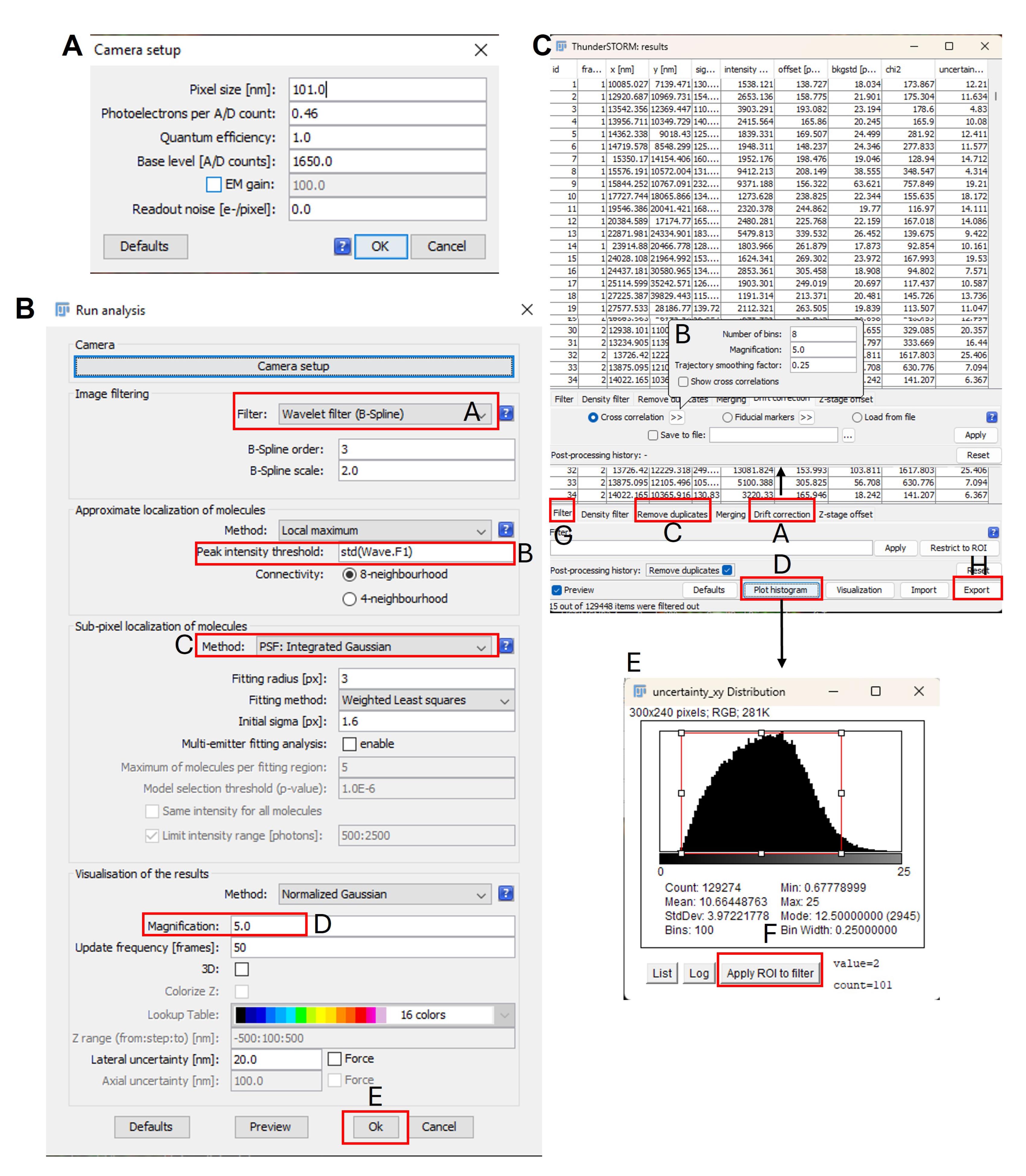
Figure 3. Summary of image reconstruction and post-processing steps using the ThunderSTORM Fiji plugin tool. (A) Camera settings crucial for image reconstruction. (B) ThunderSTORM reconstruction window. Crucial parameters are highlighted and summarized as follows: A, wavelet B-spline image filtering; B, peak intensity threshold; C, subpixel localization of molecules method (PSF: Integrated Gaussian); D, magnification; E, run analysis. (C) ThunderSTORM post-processing window. Crucial parameters are highlighted and summarized as follows: A, B, drift correction; C, remove duplicates; D, plot histogram; E, Uncertainty_xy plot with example of a red rectangular region of interest (ROI); F, apply to ROI filter; G, filter (essential to select apply filter); H, export command to save analysis table.
3. Start reconstruction (see Figure 3B).
a. Select wavelet B-spline image filtering.
b. Select the local maximum method for the molecule localization approximation, with connectivity of 8 and std(wave.F1) for peak intensity threshold, which estimates the noise level of the image. For the Alexa Fluor 647 channel, a manual correction factor of 2.5 was applied. For the phalloidin-Alexa Fluor 488 channel, the default threshold was used due to its lower blinking efficiency.
c. Select PSF: Integrated Gaussian for subpixel localization of molecules.
d. Select 5× magnification.
e. Click run analysis.
4. Post-processing steps, including lateral drift correction and data filtering, were performed using ThunderSTORM (see Figure 3C).
a. Select the drift correction function.
b. Click on the cross-correlation method. Adjust the number of bins value to 8.
c. Eliminate duplicates.
d. Eliminate poor localized molecules following these steps:
i. Plot uncertainty_xy and define the filter range by drawing a rectangular region of interest (ROI).
ii. Select apply the selection to filter.
iii. Select the apply command from the filter section.
e. Save image as a .tiff format from the file window of the Fiji console.
f. Save the analysis table from ThunderSTORM through the export command.
Data analysis
In order to evaluate the quality of the STORM reconstructed images, we reported that the localization uncertainty—used as a measure of molecule localization quality—was calculated by Gaussian fitting of the x and y molecule coordinates with respect to their center of mass. This parameter can be extracted from the ThunderSTORM molecule localization list by plotting the uncertainty histogram (plot histogram command) and selecting the appropriate range (in nm) as well as the binning [12]. The histogram can be saved as Tiff image, or values can be listed from the histogram and copied to GraphPad Prism, or alternatively, using any other suitable data analysis software. From these values, the mean uncertainty and its corresponding error, expressed as standard error of mean (SEM), were calculated (see Figures 4C, D and 5B, C). The localization precision was further quantified by calculating the full width half maximum (FWHM), defined as the distance between the two points at half of the maximum value of the Gaussian distribution, according to the following equations:
FWHM = 2 × 1.177 × σ
FWHM = 2.335 σ
Where σ = mean localization uncertainty.
Moreover, we evaluated the overall quality of image reconstruction using the NanoJ-SQUIRREL plugin tool that allows to calculate the resolution-scaled Pearson (RSP) coefficient. The RSP coefficient corresponds to the Pearson correlation between the reference TIRF image and the super-resolution image scaled to the same resolution [13]. The analysis was performed as follows:
a. Open the conventional TIRF image and the corresponding reconstructed STORM image in Fiji.
b. From the Fiji plugin window, click on the NanoJ-SQUIRREL plugin and select the calculate error map, RSE, and RSP options.
c. Define reference image: select standard TIRF image.
d. Define reconstructed image: select STORM image.
e. Click on run.
f. Save numerical results in Excel and images as Tiff files.
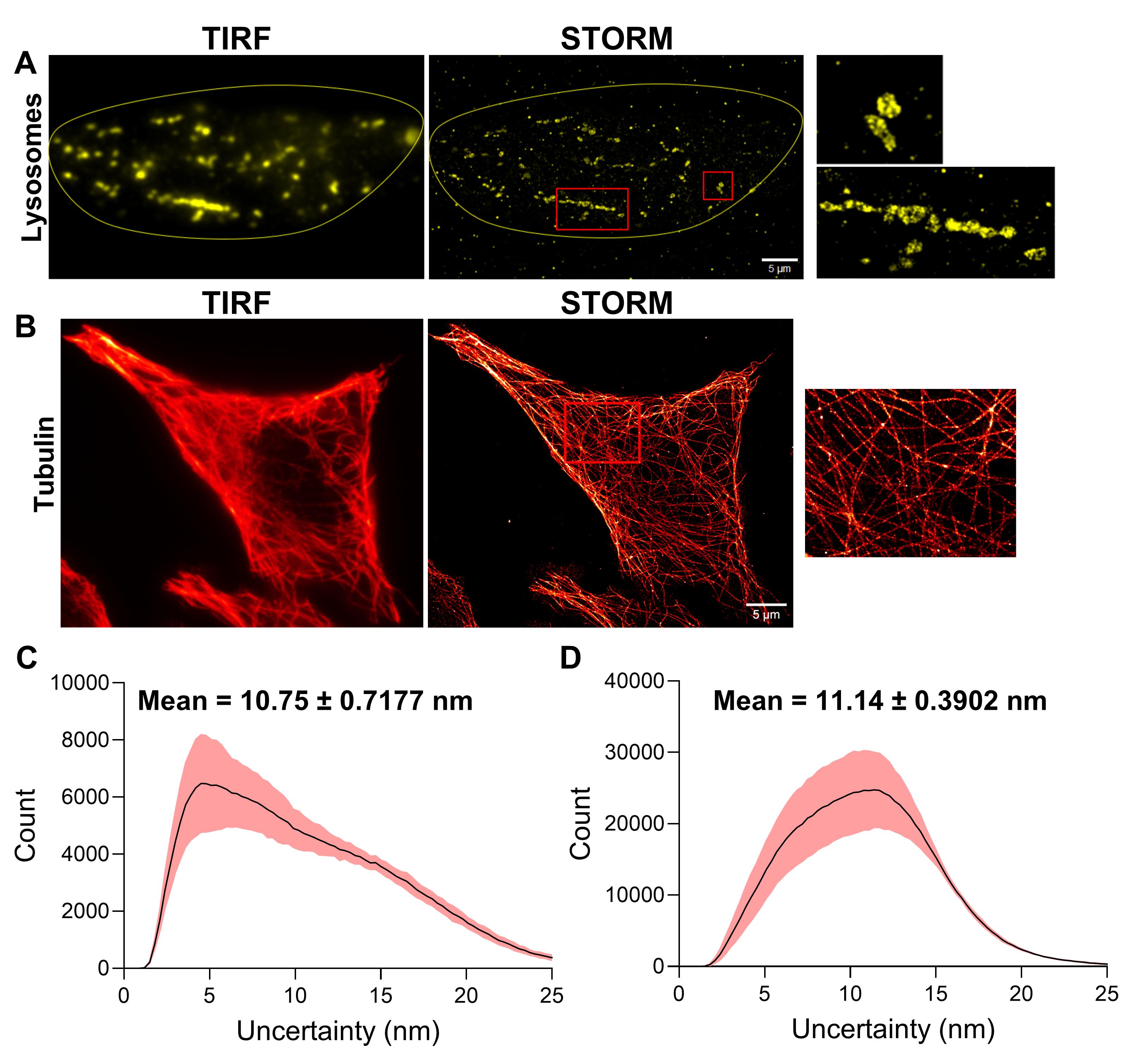
Figure 4. Lysosome and microtubules single-color stochastic optical reconstruction microscopy (STORM) reconstructions and quality assessment. (A, B) Representative total internal reflection (TIRF) and STORM images of lysosomes (A) and microtubules (B). The yellow line in the lysosome upper panel represents the cell border. Red square regions represent the magnified area presented on the right side. Scale bar, 5 μm. (C, D) Uncertainty of molecule localization, expressed in nm, of lysosomes (C) and microtubules (D). The red shadow gradients indicate the standard error of mean (SEM). Mean uncertainty ± SEM is reported on each graph. Data were obtained from three independent cells.
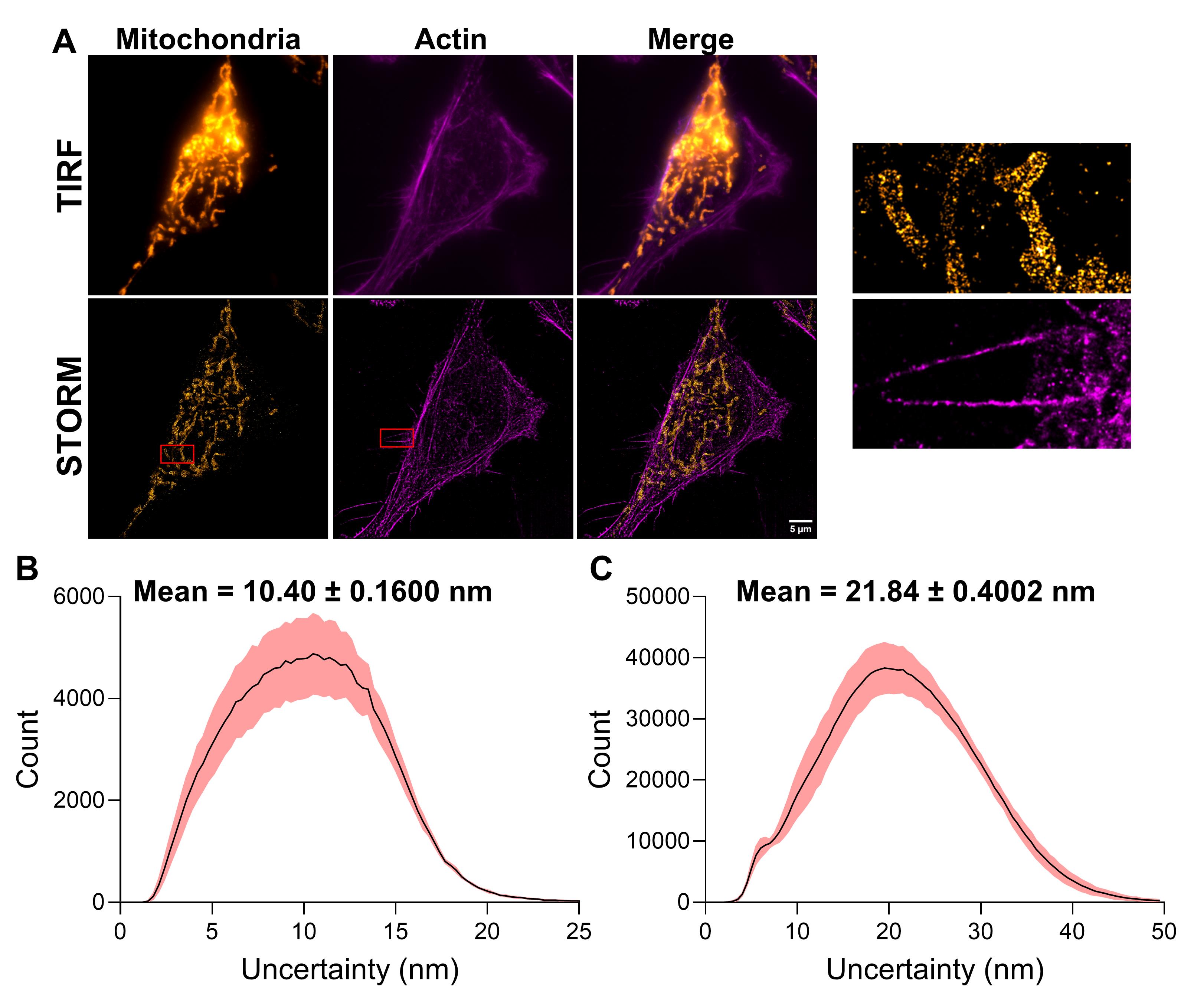
Figure 5. Mitochondria and actin cytoskeleton dual-color stochastic optical reconstruction microscopy (STORM) reconstructions and quality assessment. (A) Representative total internal reflection (TIRF) and STORM images of mitochondria, the actin cytoskeleton, and the merging of the two channels. Red square regions represent the magnified area presented on the right side. Scale bar, 5 μm. (B, C) Uncertainty of molecule localization, expressed in nm, of mitochondria (B) and actin (C). The red shadow gradients indicate the standard error of mean (SEM). Mean uncertainty ± SEM is reported on each graph. Data were obtained from three independent cells.
Validation of protocol
In order to evaluate the potential nonspecific binding of the goat-derived secondary antibodies, cells were incubated without primary and secondary antibodies to assess basal cellular autofluorescence/background (negative control) or with the secondary antibody only without the primary antibody. As shown in Figure 6, no detectable fluorescence signal was observed in the secondary antibody control condition, indicating that nonspecific binding was negligible under our blocking conditions. Moreover, no basal cellular autofluorescence/background was detected. These control experiments confirm that blocking with 10% FBS is sufficient in our experimental setup.
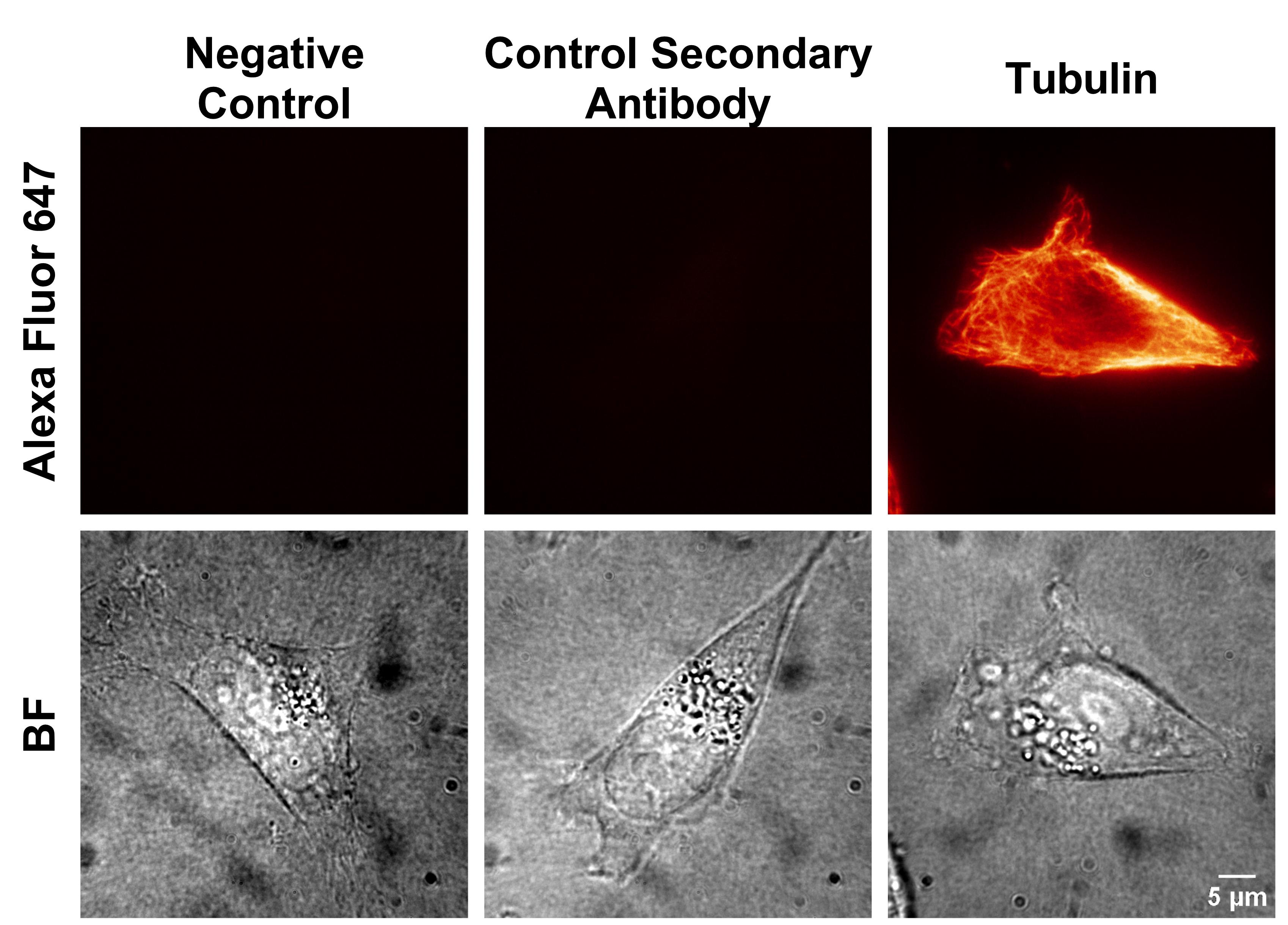
Figure 6. Control of antibody nonspecific binding. Representative total internal reflection (TIRF) images of a HeLa cell under three different experimental conditions: (i) incubated without primary and secondary antibodies to assess basal cellular autofluorescence/background (negative control); (ii) incubated with the secondary antibody only (without primary antibody) to evaluate potential nonspecific binding of the goat-derived secondary antibodies (control secondary antibody); and (iii) incubated with primary anti-tubulin and the secondary antibody (tubulin). Images were acquired using the same TIRF microscopy settings used for experimental samples and are displayed using identical grayscale intensity ranges. Scale bar, 5 μm.
The current protocol has been successfully applied to obtain high-quality single-color STORM images of lysosomes and microtubules, labeled using commercial anti-LAMP2 and an anti-tubulin primary antibody, respectively. In both cases, a goat anti-mouse conjugated with Alexa Fluor 647—one of the most suitable fluorophores for STORM imaging—was used.
This performance is supported by data shown in Figure 4A, B, which compare conventional TIRF and STORM images of lysosomes and microtubules, highlighting the substantial improvement in spatial resolution achieved by single-molecule localization microscopy. The magnified regions reveal well-preserved lysosomal structures (Figure 4A), where both the limiting membrane and the organelle lumen can be clearly distinguished. Similarly, microtubules display a dense and continuous filament network (Figure 4B). As described by uncertainty_xy quantification, the quality of single-molecule localization during image reconstruction was robust and solid (Figure 4C, D). Indeed, we obtained a mean single-molecule localization uncertainty of 10.75 and 11.14 nm for lysosomes and microtubules, respectively, which is considered a high-quality range of data for STORM. The mean localization FWHM, which describes the spread of molecule localization, was 25.3 and 26.3 nm for lysosomes and microtubules, respectively (Table 1). These data indicate a strong localization precision with a good signal-to-noise ratio and, in turn, an efficient blinking process. Image reconstruction quality was further assessed with the NanoJ-SQUIRREL plugin, which gave a resolution-scaled Pearson correlation (RSP) higher than 0.8, suggesting high structural fidelity (Table 1).
Table 1. Mean localization full width half maximum (FWHM) and mean resolution-scaled Pearson (RSP) of single-color stochastic optical reconstruction microscopy (STORM) data presented in Figure 4. Detailed description for calculation of localization FWHM and RSP is presented in the data analysis section. Data were obtained from three independent cells.
| Sample | Mean localization FWHM ± SEM (nm) | Mean RSP ± SEM (A.U.) |
|---|---|---|
| Lysosomes | 25.33 ± 1.703 | 0.8450 ± 0.0420 |
| Microtubules | 26.27 ± 0.9244 | 0.8783 ± 0.0064 |
The protocol was also successfully applied to dual-color STORM imaging of mitochondria and the actin cytoskeleton. Mitochondria were labeled using a rabbit anti-TOMM22 primary antibody followed by an Alexa Fluor 647–conjugated secondary antibody, while filamentous actin was stained with phalloidin–Alexa Fluor 488. The results and statistics presented here support the robustness of this workflow and demonstrate the preservation of cellular ultrastructure. The magnified regions reveal well-preserved mitochondrial structures (Figure 5A), where both the outer mitochondrial membrane—containing the TOMM22 transporter—and the organelle lumen can be clearly resolved. In addition, the actin cytoskeleton exhibits a dense and continuous filament network, including well-defined cellular protrusions (Figure 5A). As described by uncertainty analysis, the quality of single-molecule localization during image reconstruction is robust and solid (Figure 5B, C). Indeed, we obtained a mean localization uncertainty of 10.40 and 21.84 nm for mitochondria and actin, respectively. These metrics indicate high localization precision, a favorable signal-to-noise ratio, and an efficient fluorophore blinking process. The mean localization FWHM was 24.5 and 51.5 nm for mitochondria and the actin cytoskeleton, respectively (Table 2). In the case of mitochondria, these data indicate a strong localization precision with a good signal-to-noise ratio and, in turn, an efficient blinking process. For the actin cytoskeleton, the FWHM values are higher due to the Alexa Fluor 488 blinking efficiency, which is lower than the Alexa Fluor 647 dye, which is the top choice for STORM experiments. Image reconstruction quality was further assessed with the NanoJ-SQUIRREL plugin, which gave an RSP higher than 0.8, suggesting high structural fidelity (Table 2). Of note, the RSP value of actin is 0.91, higher than that of mitochondria; this is attributed to the labeling density achieved with phalloidin, which has been used at high concentrations to allow molecule interchanging, thus supplying the poor blinking efficiency of the Alexa Fluor 488 dye.
Table 2. Mean localization full width half maximum (FWHM) and mean resolution-scaled Pearson (RSP) of dual-color STORM data presented in Figure 5. A detailed description for the calculation of localization FWHM and RSP is presented in the Data analysis section. Data were obtained from three independent cells.
| Sample | Mean localization FWHM ± SEM (nm) | Mean RSP ± SEM (A.U.) |
|---|---|---|
| Mitochondria | 24.50 ± 0.3786 | 0.8423 ± 0.0028 |
| Actin | 51.47 ± 0.9387 | 0.9147 ± 0.0072 |
General notes and troubleshooting
General notes
1. This protocol provides a robust workflow for high-quality STORM imaging of lysosomes, microtubules, mitochondria, and actin. After optimization, adaptability, and troubleshooting of specific reagents and conditions, this method is broadly applicable [13]. Detailed reporting of reagent preparation, storage conditions, and stability is critical to ensure experimental reproducibility and reliable protocol implementation across laboratories [13].
2. The protocol has been validated in HeLa cells; however, it is expected to also work in other adherent cell lines. Fixation and permeabilization may vary between cell types; thus, optimization of fixation/permeabilization solutions and incubation times may be required.
3. The protocol is also expected to be applicable to other cellular structures (e.g., Golgi, endoplasmic reticulum, nucleus), provided that a high-quality primary antibody is available. For new labeling experiments, optimization of antibody concentration, blocking conditions, and incubation steps is recommended.
4. For optimal STORM reconstruction, the effective fluorophore density should allow sufficient sampling of the underlying structure while maintaining sparse activation. Typically, this corresponds to approximately one emitting molecule per diffraction-limited area in each imaging frame, to prevent spatial overlap and ensure accurate single-molecule localization.
Troubleshooting
Problem 1: No bleaching of the fluorophore or poor blinking events.
Possible cause: Buffer composition.
Solutions: Prepare a fresh buffer or revise buffer components, especially enzymes.
Problem 2: Low molecule number or discontinuous structures.
Possible cause: Low labeling efficiency.
Solution: Optimize primary antibody dilution and labeling protocol.
Problem 3: Problem with drift correction.
Possible cause: High drift.
Solutions: Try to increase bins number to 10. Sometimes, the plugin gets stacked; try to restart Fiji.
Problem 4: Problem with noisy data or a low number of detected molecules for Alexa Fluor 647.
Possible cause: Blinking density.
Solution: Try to adjust the threshold standard deviation (std)(wave.F1) correction factor. If data are noisy, try to increase the correction factor to 3 or 3.5, without exceeding 4, which can lead to missing real molecules. On the other hand, for a poor molecule detection, try to remove the correcting factor or decrease the number to 2 or 1.5. Compare the different conditions by looking at the images’ background and structure of interest, molecule number in the resulting table list, uncertainty, and quality control with NanoJSQUIRREL.
Molecule counts are expected to vary depending on the labeled cellular structure. For tubulin and mitochondria labeled with Alexa Fluor 647 secondary antibody, the number of detected molecules is typically in the range of 1.2–1.5 × 10⁶ molecules. In contrast, lysosomes labeled with Alexa Fluor 647 secondary antibodies exhibit fewer detected molecules, approximately 0.25 × 10⁵, due to their smaller size, morphology, and localization within a restricted cytoplasmic region. For actin labeled with phalloidin Alexa Fluor 488, the expected number of detected molecules is approximately 1.5 × 10⁶, which can be attributed to the relatively high phalloidin concentration used for the staining, to allow molecule interchanging.
Regarding localization precision, samples labeled with Alexa Fluor 647 typically exhibit uncertainty values in the range of 10–20 nm, indicating very high localization accuracy. In comparison, samples labeled with Alexa Fluor 488 generally show uncertainty values around 20–30 nm, reflecting the moderate blinking behavior and lower brightness of Alexa Fluor 488 compared with Alexa Fluor 647.
Acknowledgments
G.D. and A.O.B. conceptualized and supervised the study. G.D. and J.F.C. performed the protocol and analyzed the data. G.D. wrote the original draft. G.D., A.O.B., and J.F.C. contributed to the manuscript review and editing.
We acknowledge financial support from the Spanish State Research Agency, MICIU/AEI/10.13039/501100011033, through the “Severo Ochoa” Programme for Centers of Excellence in R&D: CEX2023-001386-S.
We acknowledge Francisco Porto from Leica Microsystem for technical support essential for imaging acquisition.
Competing interests
The authors declare no conflicts of interest.
References
- Gray, N. (2009). Knowing the limit. Nat Cell Biol. 11: S8–S8. https://doi.org/10.1038/ncb1940
- Huang, B., Bates, M. and Zhuang, X. (2009). Super-Resolution Fluorescence Microscopy. Annu Rev Biochem. 78: 993–1016. https://doi.org/10.1146/annurev.biochem.77.061906.092014
- Lelek, M., Gyparaki, M. T., Beliu, G., Schueder, F., Griffié, J., Manley, S., Jungmann, R., Sauer, M., Lakadamyali, M., Zimmer, C., et al. (2021). Single-molecule localization microscopy. Nat Rev Methods Primers. 1(1): 39. https://doi.org/10.1038/s43586-021-00038-x
- Betzig, E., Patterson, G. H., Sougrat, R., Lindwasser, O. W., Olenych, S., Bonifacino, J. S., Davidson, M. W., Lippincott-Schwartz, J. and Hess, H. F. (2006). Imaging Intracellular Fluorescent Proteins at Nanometer Resolution. Science. 313(5793): 1642–1645. https://doi.org/10.1126/science.1127344
- Sigal, Y. M., Zhou, R. and Zhuang, X. (2018). Visualizing and discovering cellular structures with super-resolution microscopy. Science. 361(6405): 880–887. https://doi.org/10.1126/science.aau1044
- Bates, M., Huang, B., Dempsey, G. T. and Zhuang, X. (2007). Multicolor Super-Resolution Imaging with Photo-Switchable Fluorescent Probes. Science. 317(5845): 1749–1753. https://doi.org/10.1126/science.1146598
- Huang, B., Wang, W., Bates, M. and Zhuang, X. (2008). Three-Dimensional Super-Resolution Imaging by Stochastic Optical Reconstruction Microscopy. Science. 319(5864): 810–813. https://doi.org/10.1126/science.1153529
- Dani, A., Huang, B., Bergan, J., Dulac, C. and Zhuang, X. (2010). Superresolution Imaging of Chemical Synapses in the Brain. Neuron. 68(5): 843–856. https://doi.org/10.1016/j.neuron.2010.11.021
- Xu, K., Zhong, G. and Zhuang, X. (2013). Actin, Spectrin, and Associated Proteins Form a Periodic Cytoskeletal Structure in Axons. Science. 339(6118): 452–456. https://doi.org/10.1126/science.1232251
- Rust, M. J., Bates, M. and Zhuang, X. (2006). Sub-diffraction-limit imaging by stochastic optical reconstruction microscopy (STORM). Nat Methods. 3(10): 793–796. https://doi.org/10.1038/nmeth929
- Tuladhar, A., Guffroy, M., Finnema, S. J., Christmann, R., Van Vleet, T. R., Mayana, S. A. K. and Fossey, S. (2025). Investigation of bone toxicity in drug development: review of current and emerging technologies. Toxicol Sci. 208(2): 207–224. https://doi.org/10.1093/toxsci/kfaf131
- Lehmann, M., Lichtner, G., Klenz, H. and Schmoranzer, J. (2015). Novel organic dyes for multicolor localization-based super-resolution microscopy. J Biophotonics. 9: 161–170. https://doi.org/10.1002/jbio.201500119
- Yu, K., Tuladhar, A., Dankberg, S., Dai, C. and McGee-Lawrence, M. E. (2025). Integrating 3D Osteocyte Culture, Microgravity Simulation, and Fluid Flow Reveals Mechanisms of Osteocyte Mechanosensation and Calcium Signaling Altered by Disuse. Biomolecules. 15(11): 1534. https://doi.org/10.3390/biom15111534
- Fish, K. N. (2022). Total Internal Reflection Fluorescence (TIRF) Microscopy. Curr Protocol. 2(8): e517. https://doi.org/10.1002/cpz1.517
- Ovesný, M., Křížek, P., Borkovec, J., Švindrych, Z. and Hagen, G. M. (2014). ThunderSTORM: a comprehensive ImageJ plug-in for PALM and STORM data analysis and super-resolution imaging. Bioinformatics. 30(16): 2389–2390. https://doi.org/10.1093/bioinformatics/btu202
- Culley, S., Albrecht, D., Jacobs, C., Pereira, P. M., Leterrier, C., Mercer, J. and Henriques, R. (2018). Quantitative mapping and minimization of super-resolution optical imaging artifacts. Nat Methods. 15: 263–266. https://doi.org/10.1038/nmeth.4605
- Tuladhar, A., Shaver, J. C., McGee, W. A., Yu, K., Dorn, J., Horne, J. L., Alhamad, D. W., Hagan, M. L., Cooley, M. A., Zhong, R., et al. (2024). Prkd1 regulates the formation and repair of plasma membrane disruptions (PMD) in osteocytes. Bone. 186: 117147. https://doi.org/10.1016/j.bone.2024.117147
Article Information
Publication history
Received: Jan 30, 2026
Accepted: Mar 22, 2026
Available online: Apr 10, 2026
Published: Apr 20, 2026
Copyright
© 2026 The Author(s); This is an open access article under the CC BY-NC license (https://creativecommons.org/licenses/by-nc/4.0/).
How to cite
Fernández de Córdoba, J., Oña, A. and D’Agostino, G. (2026). Accessible STORM Imaging: An Optimized Workflow for Conventional Widefield Epifluorescence/TIRF Setups. Bio-protocol 16(8): e5672. DOI: 10.21769/BioProtoc.5672.

 Download Citation in RIS Format
Category
Biophysics > Microscopy > Single-molecule localization microscopy
Cell Biology > Cell imaging > Super resolution imaging
Cell Biology > Cell imaging > Widefield microscopy
Do you have any questions about this protocol?
Post your question to gather feedback from the community. We will also invite the authors of this article to respond.
 Post a Question


