- Protocols

- Articles and Issues
- For Authors
- About
- Become a Reviewer

A Bioinformatics Workflow to Identify eccDNA Using ECCFP From Long-Read Nanopore Sequencing Data
(*contributed equally to this work) Published: Vol 16, Iss 6, Mar 20, 2026 DOI: 10.21769/BioProtoc.5636 Views: 15
Reviewed by: Migla MiskinyteYuhang WangAnonymous reviewer(s)
Original research article
The authors used this protocol in:

Feb 2026

Protocol Collections
Comprehensive collections of detailed, peer-reviewed protocols focusing on specific topics


Abstract
Extrachromosomal circular DNA (eccDNA) is a type of circular DNA that exists independently of chromosomes and has garnered significant attention in various fields, particularly in the context of smaller eccDNAs, which have considerable roles in gene regulation through various mechanisms. Current methods such as Circle-Seq and 3SEP can enrich small eccDNAs during sample preparation, but most bioinformatics pipelines remain challenging, exhibiting low accuracy and efficiency. This protocol describes the detailed workflow of a newly developed bioinformatics analysis pipeline, named EccDNA Caller based on Consecutive Full Pass (ECCFP), to accurately identify eccDNA from long-read Nanopore sequencing data. Compared to other pipelines, ECCFP significantly improves detection sensitivity, accuracy, and runtime efficiency. The process includes raw data quality control, trimming of adapters and barcodes, alignment to a reference genome, and identification of eccDNA, with detailed results encompassing accurate positioning of eccDNA, consensus sequences, and variants of individual eccDNA.
Key features
• This protocol provides a beginner-friendly, step-by-step workflow that enables researchers without bioinformatics experience to successfully execute the entire eccDNA identification process.
• It offers an efficient computational pipeline for eccDNA detection from Nanopore sequencing data, integrating quality control, trimming, alignment, and eccDNA identification.
• ECCFP exhibits sensitivity, accuracy, high efficiency, and low false-positive rates compared to existing long-read-based tools.
Keywords: ECCFPGraphical overview
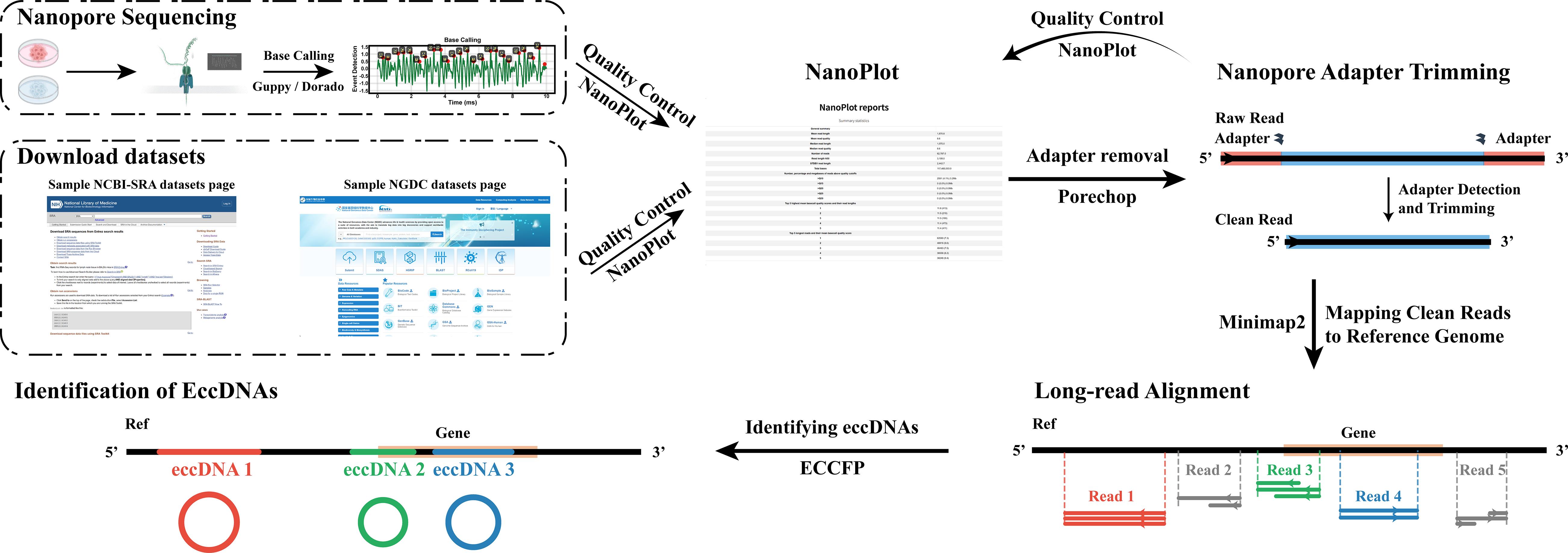
The entire process from Nanopore sequencing data acquisition to eccDNA identification
Background
Extrachromosomal circular DNA (eccDNA) is a type of genetic material that exists independently of chromosomes and is widely found in eukaryotic organisms [1,2]. Recent studies have highlighted its significant role in various biological functions, particularly in cancer initiation, progression, and drug resistance [3–6]. In addition, eccDNA varies from tens to millions of base pairs (bp) in length, where molecules exceeding 10 kb are classified as ecDNA [7]. These large circular DNA molecules have been identified in over half of all human cancers, primarily using FISH and whole-genome sequencing (WGS) for validation [8,9]. Current experimental methods developed for the enrichment of small eccDNA, such as Circle-Seq [10] and 3SEP [11,12], typically identify eccDNA molecules smaller than 10 kb. These smaller eccDNA molecules have been demonstrated to regulate gene expression through various mechanisms [13].
Both Circle-Seq and 3SEP experimental methodologies utilize rolling circle amplification (RCA). During RCA, DNA polymerase continually traverses circular templates, producing concatemeric tandem copies (CTCs) [14]. Currently, most bioinformatics pipelines for eccDNA detection are based on overly strict selection criteria for CTCs [15] and often overlook the complexities introduced by rolling circle amplification (RCA) and random errors during the sequencing process, which might result in ghost sequences.
Recently, our group developed a novel bioinformatics pipeline, named EccDNA Caller based on Consecutive Full Pass (ECCFP) [16], for eccDNA detection from long-read Nanopore sequencing data. ECCFP utilizes all individual sequencing reads, including ghost and non-ghost sequences, to identify candidate eccDNA molecules. The pipeline then integrates these candidate eccDNAs and employs the Boyer–Moore majority vote algorithm to accurately determine eccDNA positions and gather information on circular consensus sequences. Compared to other current pipelines that identify small eccDNA molecules from long-read sequencing data using RCA amplification, ECCFP combines the strengths of these pipelines and is optimized specifically for RCA data, resulting in improved sensitivity, accuracy, and operational efficiency.
Briefly, the current signal data from Nanopore sequencing, typically stored in FAST5 or POD5 formats, undergo base calling through tools such as Guppy or Dorado. This computational conversion transforms the current signal data into nucleotide sequence data, ultimately producing demultiplexed FASTQ files for downstream genomic analyses. Upon FASTQ acquisition, initial quality assessment is performed using NanoPlot. Adapter and barcode sequences are then removed with Porechop, followed by post-trimming quality re-evaluation of trimmed reads using NanoPlot. Trimmed reads require alignment to a reference genome for sequence mapping. Minimap2 serves as the optimal aligner for long-read data due to its efficient handling of error-prone sequences. Subsequent eccDNA detection is conducted using ECCFP, which identifies circular DNA through structural signature analysis of aligned reads. The entire process from Nanopore sequencing data acquisition to eccDNA identification can be referenced to in the Graphical Overview for clearer understanding. This protocol details the core bioinformatic workflow for eccDNA detection, encompassing quality control, adapter and barcode trimming, reference genome alignment, and circular DNA identification. As a computational pipeline, it exclusively addresses analytical methodologies while explicitly excluding wet laboratory procedures. All sequencing data used are derived from public repositories, including Project PRJCA040952 and PRJCA052047 deposited by our group at NGDC alongside datasets from published studies.
This protocol relies exclusively on open-source software tools that are readily accessible. Furthermore, we provide comprehensively documented analytical code designed to guide users through the complete workflow from FASTQ processing to eccDNA identification. This makes the protocol accessible even for researchers without prior bioinformatics experience.
Software and datasets
Hardware
The analysis was performed on a Linux/Unix system in the following benchmarked configuration:
1. Memory (RAM): 512 GB
2. CPU: 64-bit architecture, 18 cores, 72 threads
Note: This setup demonstrates robust performance for the entire workflow. Hardware specifications can be adjusted based on data scale and resource availability.
Software
1. Conda (version 24.9.2, https://anaconda.org/anaconda/conda)
2. Python (version 3.12.2, https://www.python.org/downloads/)
3. ECCFP (version 1.0.1, https://github.com/WSG-Lab/ECCFP, MIT License)
4. Porechop (version 0.2.4, https://github.com/rrwick/Porechop, GNU General Public License v3.0)
5. Minimap2 (version 2.28, https://github.com/lh3/minimap2, MIT License) [17,18]
6. NanoPlot (version 1.42.0, https://github.com/wdecoster/NanoPlot, MIT License) [19]
Note: Conda is used as the package manager and Python as the interpreter. Although there are no absolute version requirements, to ensure reproducibility of the environment and avoid compatibility issues, we strongly recommend using the above suggested version combinations.
Software requirements: dependencies
1. numpy (version 1.26.4, https://numpy.org/)
2. pandas (version 2.3.2, https://pandas.pydata.org/ )
3. rich (version 14.1.0, https://rich.readthedocs.io/ )
4. biopython (version 1.85, https://biopython.org/)
5. pyfaidx (version 0.9.0.1, https://github.com/mdshw5/pyfaidx)
6. pyfastx (version 2.2.0, https://github.com/lmdu/pyfastx) [20]
Note: Although specific versions are listed for completeness, only minimap2, numpy, pandas, and biopython have strict version requirements. While version inconsistencies in other tools are unlikely to critically impact results, we strongly recommend maintaining a consistent software environment to ensure full reproducibility and computational stability.
Data
All sequencing data generated and analyzed in this study are publicly accessible through the National Genomics Data Center (NGDC) and the NCBI Sequence Read Archive (SRA). Specifically, the NGDC hosts data under project accessions PRJCA040952 and PRJCA052047 (generated and deposited by our laboratory; access requires an application to the database) as well as PRJCA010264. Detailed application guidelines for PRJCA040952 are provided in the official documentation ( https://ngdc.cncb.ac.cn/gsa-human/document/GSA-Human_Request_Guide_for_Users_us.pdf) and are not reiterated here. Data are available from the NCBI SRA under project accession PRJNA806866, from which the following four sample IDs were utilized: SRR18143375, SRR18143376, SRR18143377, and SRR18143378 (Table 1). All analyzed samples originated from human cell lines. Genomic alignments and subsequent analyses were based on the GRCh38.p14 (hg38) reference genome assembly obtained from the GENCODE database.
Table 1. Summary of publicly available sequencing datasets
| Project | Data_id | Sample |
|---|---|---|
| PRJCA040952 | HRR2590080 | HepG2 cell |
| PRJCA010264 | HRR695439 | BGC823 cell |
| PRJCA010264 | HRR695440 | SGC7901 cell |
| PRJCA010264 | HRR695441 | GES1 cell |
| PRJCA010264 | HRR695442 | HepG2 cell |
| PRJCA010264 | HRR695443 | HL7702 cell |
| PRJCA010264 | HRR695444 | MDA-MB-453 cell |
| PRJCA010264 | HRR695445 | MCF12A cell |
| PRJNA806866 | SRR18143375 | EJM cells |
| PRJNA806866 | SRR18143376 | JJN3 cell |
| PRJNA806866 | SRR18143377 | APR1 cell |
| PRJNA806866 | SRR18143378 | APR1 cell |
Procedure
A. Create the analysis environment
All analyses in this protocol are performed within the Linux terminal, which is used to install software, download data, and execute computational workflows. This section describes the initial setup of software dependencies and the dedicated Conda environment required for the analysis.
Conda is used to establish an isolated virtual environment for this workflow, ensuring reproducibility and preventing software conflicts between projects. To install Conda, visit the official website (https://anaconda.org/), click Download (usually found in the top-right corner), and select the appropriate installer for your operating system ("Anaconda Distribution" for full support or "Miniconda" for a minimal installation). After downloading, run the installation script and follow the prompts to complete the setup (on some systems, execution permissions may need to be assigned to the script first).
In the command-line instructions below, lines beginning with a “#” are comments that describe the purpose of the subsequent commands and are not executed by the terminal. The above steps can also be performed via terminal commands. The commands for a typical installation on a Linux system are provided below:
# Download the Anaconda installation script.wget https://repo.anaconda.com/archive/Anaconda3-2024.10-1-Linux-x86_64.sh # Make the script executable.chmod +x Anaconda3-2024.10-1-Linux-x86_64.sh# Run the installation script../Anaconda3-2024.10-1-Linux-x86_64.sh# Verify software is installed.conda --versionA successful installation is confirmed if the command conda --version returns a version number (e.g., conda 24.9.2). If the command is not found or an error is returned, review the terminal output from the installation script for specific error messages to diagnose the issue.
Following a successful Conda installation, an isolated virtual environment named eccfpEnv must be created to manage all software dependencies for this workflow. All subsequent analyses will be conducted within this activated environment. Execute the following commands in your terminal:
# Create a new conda environment named 'eccfpEnv'.conda create -n eccfpEnv -y# List all available conda environments to verify creation.conda env list# Activate the newly created 'eccfpEnv' environment.conda activate eccfpEnv# =====================================================================# All subsequent analyses are performed within the eccfpEnv environment# =====================================================================# (Optional) To later deactivate the current environment.# conda deactivate
Successful creation and activation of the eccfpEnv environment completes section A. For readers who may be unfamiliar with the Linux operating system, basic command references are available at https://ubuntu.com/tutorials/command-line-for-beginners#1-overview.
To minimize issues arising from system variations, all subsequent steps will be performed within a standardized directory structure. The setup is as follows: first, create a directory named “eccfpws” in the user’s home directory to store all subsequent files and serve as the main working directory. Then, within this directory, create three subdirectories named “Software,” “RawData,” and “Reference” to store the software tools required by this protocol, the FASTQ sequencing files, and the reference genome file, respectively. The code used is as follows:
cd ~# cd: a shell command to change the shell working directory.# ~: Symbol represents the current user's home directory (typically /home/username on Linux).# The shell command 'cd ~' changes the current working directory to the user's home directory.mkdir eccfpws# mkdir: a shell command to create new directories (make directory).# This command creates a new directory named "eccfpws" in the current location.mkdir eccfpws/RawData eccfpws/Reference eccfpws/Software# This command creates three subdirectories (RawData, Reference, and Software)# Simultaneously within the eccfpws directory.cd eccfpws# This command changes the current working directory to the newly created eccfpws directory.B. Software and dependency installation
With the eccfpEnv environment activated, the next step involves installing the necessary software and dependency packages to proceed with the subsequent analysis. The required dependencies and some software can be installed via Conda or Python. First, install Python, numpy, pandas, and rich using Conda with the following command code:
# Activate conda environment.conda activate eccfpEnv# Install Python packages with specific versions.conda install -y python=3.12.2 numpy=1.26.4 pandas=2.3.2 rich=14.1.0# List installed packages to verify installation.conda list# Check Python version to confirm successful installation.python --versionFollowing successful Python installation, proceed to install the additional packages required for ECCFP operation, biopython, pyfaidx, and pyfastx, using the following commands in the terminal:
# Install essential Python dependencies for ECCFP.pip install biopython==1.85 pyfaidx==0.9.0.1 pyfastx==2.2.0# Confirm package installation.pip listAfter confirming successful installation of all required packages, proceed to install the analysis software. Installation methods vary considerably between tools: ECCFP and Porechop require installation from GitHub source code; NanoPlot can be installed directly through Conda or pip; and Minimap2 is available as pre-compiled binaries on GitHub, requiring no installation beyond downloading. To maintain organizational structure, execute all following commands within the previously created eccfpws/Software directory:
# Navigate to the software directorycd ~/eccfpws/Software# Install ECCFP from sourcegit clone https://github.com/WSG-Lab/ECCFP.gitcd ECCFPconda env update -f environment.ymlpip install .eccfp --help # Verify installation and display help message# Install Porechop from sourcecd ..git clone https://github.com/rrwick/Porechop.gitcd Porechoppython3 setup.py installporechop -h # Verify installation and display help message# Install NanoPlotconda install -c bioconda nanoplot# Alternative installation method: pip install NanoPlotNanoPlot --help # Verify installation and display help messageThe installation for Minimap2 differs from the other tools as it is provided as a pre-compiled binary. Unlike packages installed via pip or Conda, the Minimap2 executable is not automatically added to your system's PATH. Therefore, to run it simply by typing Minimap2, you need to manually place it in a directory that is included in your PATH. A recommended approach is to create a symbolic link (functionally equivalent to a Windows shortcut) within your active Conda environment's bin directory, which is already in the PATH.
You can verify that the eccfp command is properly located in this directory by using which eccfp. The following steps outline this process:
# Return to the sortware directorycd ~/eccfpws/Software# Download and extract minimap2wget https://github.com/lh3/minimap2/releases/download/v2.28/minimap2-2.28_x64-linux.tar.bz2tar -jxvf minimap2-2.28_x64-linux.tar.bz2# Test the executable~/eccfpws/Software/minimap2-2.28_x64-linux/minimap2 --help# Identify your Conda environment's bin directory (where eccfp was installed)which eccfp# This will return a path like:# output: /home/username/anaconda3/envs/eccfpEnv/bin/eccfp# NOTE: Your exact path will differ. Use the output from this command.# Create a symbolic link to minimap2 in that bin directory# Replace '/home/username/anaconda3/envs/eccfpEnv/bin' with the path from 'which eccfp'ln -s ~/eccfpws/Software/minimap2-2.28_x64-linux/minimap2 ~/anaconda3/envs/eccfpEnv/bin/# Verify minimap2 is now accessibleminimap2 --helpAll core analysis software has now been installed. This section covers the optional install of SRA-Toolkit (v3.2.1), which is used specifically for downloading data from NCBI. If your sequencing data is already available through alternative sources, this step may be skipped. To install, simply download the appropriate binary from the official repository, extract the archive, and add the prefetch and fasterq-dump executables to your system PATH to enable sequencing data retrieval and format conversion in subsequent steps.
# Return to the sortware directorycd ~/eccfpws/Software# Code for installing SRA-Toolkit# Download and install SRA-Toolkitwget https://ftp-trace.ncbi.nlm.nih.gov/sra/sdk/3.2.1/sratoolkit.3.2.1-ubuntu64.tar.gztar -xzvf sratoolkit.3.2.1-ubuntu64.tar.gzwhich eccfp# output: /home/username/anaconda3/envs/eccfpEnv/bin/eccfpln -s ~/eccfpws/Software/sratoolkit.3.2.1-ubuntu64/bin/prefetch ~/anaconda3/envs/eccfpEnv/bin/ln -s ~/eccfpws/Software/sratoolkit.3.2.1-ubuntu64/bin/fasterq-dump ~/anaconda3/envs/eccfpEnv/bin/prefetch --helpfasterq-dump --helpC. Data preparation
The sequencing data utilized in this protocol are publicly available from the NGDC and NCBI SRA. The reference genome data (hg38, GRCh38.p14) was obtained from the GENCODE database.
To download data from the NGDC:
1. Navigate to the NGDC website: https://ngdc.cncb.ac.cn/.
2. In the search bar, click All Databases, select NGDC Databases, and then choose BioProject.
3. Enter either “PRJCA040952” or “PRJCA010264” into the search box.
4. Initiate the search.
5. Once the project page loads, click on the respective GSA-Human accession number: “HRA011726” for PRJCA040952 or “HRA002605” for PRJCA010264.
6. This leads to the data access page. To request the data, click the “Request Data” button and follow the official application guidelines available at https://ngdc.cncb.ac.cn/gsa-human/document/GSA-Human_Request_Guide_for_Users_us.pdf
Upon successful application, NGDC will provide download links. Once downloaded, move the data files to the RawData directory using the mv command, or create symbolic links to them in the RawData directory using the ln -s command.
# Renames a filemv old-filename new-filename# Moves a file from its current location to the target directorymv /path/filename /target-folder/# Creates a symbolic link to the file within the RawData directoryln -s /path/filename ~/eccfpws/RawDataThe dataset used from NCBI SRA is under project accession PRJNA806866. This protocol specifically utilizes the following four samples from this project: SRR18143375, SRR18143376, SRR18143377, and SRR18143378. These datasets can be downloaded using the prefetch tool from SRA-Toolkit, followed by conversion of the downloaded SRA files to FASTQ format using fasterq-dump .
The SRA format is a compressed binary format used by NCBI to archive sequencing data. To use these data in downstream analyses, they must be converted to FASTQ format using tools such as fasterq-dump.
Code for downloading and converting Project PRJNA806866 data:
# Navigate to the RawData directorycd ~/eccfpws/RawData# Download the specified SRA datasetsprefetch SRR18143375 SRR18143376 SRR18143377 SRR18143378 -O .# Convert downloaded SRA files to FASTQ format# Note: It is recommended to use a loop for batch processing multiple filesfasterq-dump --threads 16 SRR18143375/SRR18143375.sra -O .# Batch conversion example using a loop:ls | grep -v '\.' | grep SRR | while read srrdo fasterq-dump --threads 16 ${srr}/${srr}.sra -O .doneNote: The prefetch command will create individual directories for each SRA accession (SRR18143375, SRR18143376, etc.) containing the corresponding SRA files. The fasterq-dump command then processes these SRA files to generate FASTQ format files in the current directory.
All data in these projects are human-derived. This protocol uses the hg38 (GRCh38.p14) reference genome from GENCODE.
Download steps:
1. Go to https://www.gencodegenes.org/
2. Select HUMAN → Current release
3. Under “Fasta files,” choose Genome sequence (GRCh38.p14) + ALL Regions
4. Click Fasta to download
5. Move GRCh38.p14.genome.fa to ~/eccfpws/Reference for analysis
# Navigate to the RawData directorycd ~/eccfpws/Reference# Download the GRCh38.p14 genome (compressed)wget https://ftp.ebi.ac.uk/pub/databases/gencode/Gencode_human/release_49/GRCh38.p14.genome.fa.gz# Decompress the filegunzip GRCh38.p14.genome.fa.gzD. Data quality control using NanoPlot
NanoPlot evaluates the quality of Nanopore sequencing data by generating various plots and summary statistics, providing insights into data quality and distribution. When using NanoPlot, a FASTQ-formatted sequencing reads file is required, and the final quality assessment results are primarily presented in NanoPlot-report.html.
First, create a directory named 01QualityControl to store all results. When performing quality control on multiple samples, use a for loop to process all sequencing files in the RawData directory:
cd ~/eccfpwsmkdir 01QualityControlls RawData/*.fastq RawData/*.fq 2>/dev/null | while read fastqdo if [[ "$fastq" == *.fastq ]]; then prefix=$(basename ${fastq} .fastq) elif [[ "$fastq" == *.fq ]]; then prefix=$(basename "$fastq" .fq) else echo "Warning: Unknown file extension for $(basename "$fastq")" echo "Supported formats: .fastq, .fq" fi NanoPlot --fastq ${fastq} -o 01QualityControl/${prefix} -t 16 --plots hex dotDoneWhen using a single sample:
# Example for a single sample (e.g., HRR2590080 from PRJCA040952)NanoPlot --fastq RawData/HRR2590080.fastq -o 01QualityControl/HRR2590080 -t 16 --plots hex dotNote: The command 2>/dev/null suppresses error messages when one of the file patterns does not match any files. The sed command handles both. fastq and. fq extensions when creating the output directory name.
For each sample processed, NanoPlot generates a dedicated output directory. The primary results are compiled within an interactive NanoPlot-report.html file, which can be opened in any web browser for detailed inspection. Using sample HRR2590080 as an example, the following section outlines the report structure and provides key interpretations.
The report first presents a Summary Statistics section (Figure 1), providing a high-level quantitative overview. This section includes:
• General Summary: Core statistics such as the total number of reads, total gigabases sequenced, and the N50 value.
• Reads Above Quality Cutoffs: The number, percentage, and total megabases of reads that exceed defined quality thresholds, useful for assessing the proportion of high-quality data.
• Top 5 Reads by Quality: The five reads with the highest mean basecall quality scores and their respective lengths, highlighting the best-quality data.
• Top 5 Longest Reads: The five longest reads and their mean basecall quality scores, identifying the longest fragments sequenced.
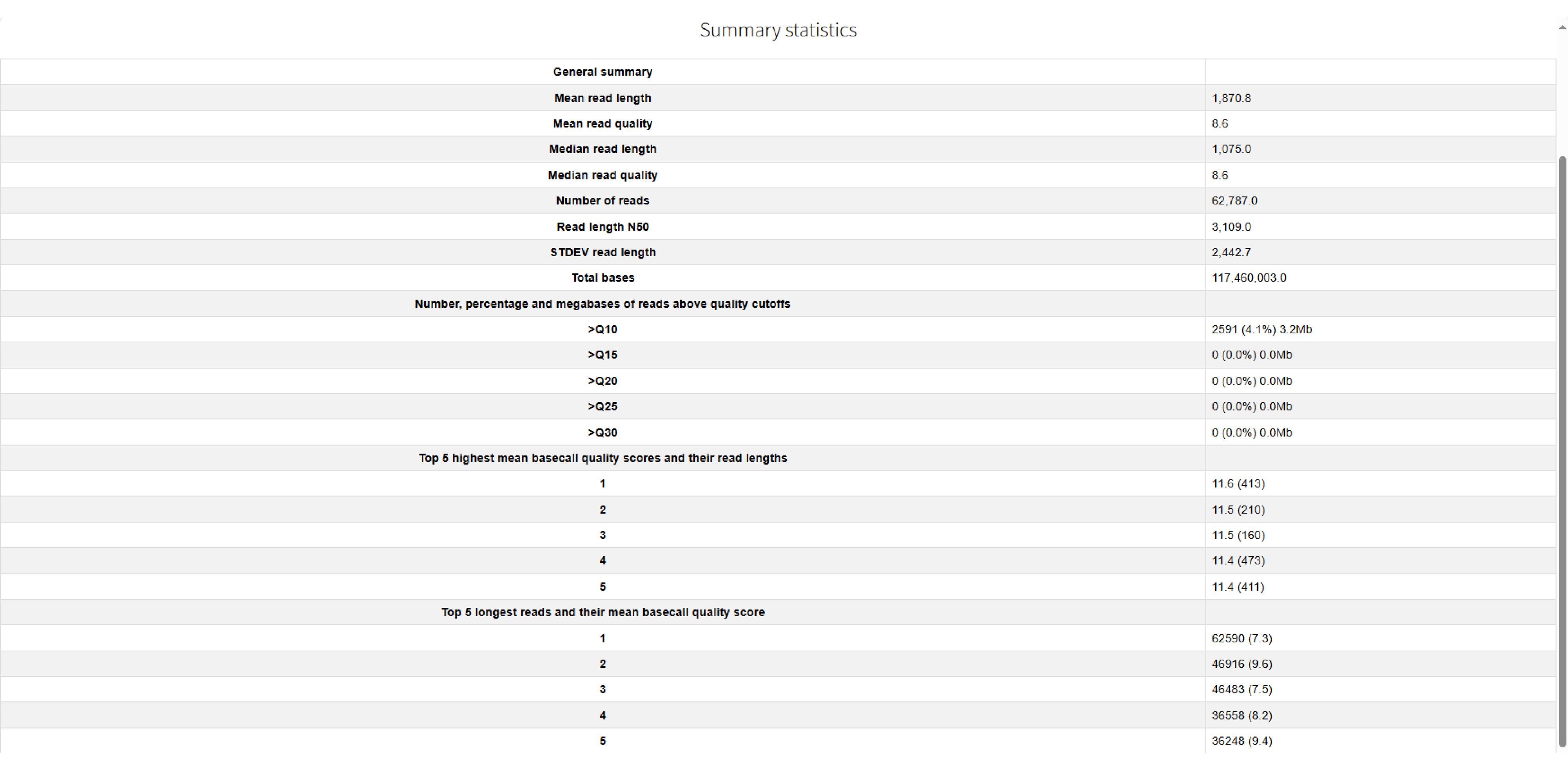
Figure 1. Summary of NanoPlot quality control results for the HRR2590080
The report is supplemented by several key visualizations (Figure 2):
• Non-Weighted Histogram of Read Lengths (Log Transformed) (Figure 2A): This plot displays the distribution of read lengths on a logarithmic x-axis (read length) against the frequency on the y-axis (number of reads). It visualizes the fragment size distribution in the sample. In ideal scenarios, this distribution often approximates a log-normal distribution, indicating a healthy sample without significant degradation.
• Read Length vs. Average Read Quality Dot Plot (Figure 2B): This scatter plot explores the relationship between read length (x-axis) and its corresponding average quality score (y-axis). It is a critical diagnostic tool for identifying issues such as DNA degradation, which often manifests as a trend where longer reads exhibit lower quality.
• Yield by Length (Figure 2C): This plot illustrates the cumulative sequencing output (yield) relative to read length. It helps visualize the proportion of the total data comprised by reads of certain lengths, showing how much of the total sequence is contained within long fragments.
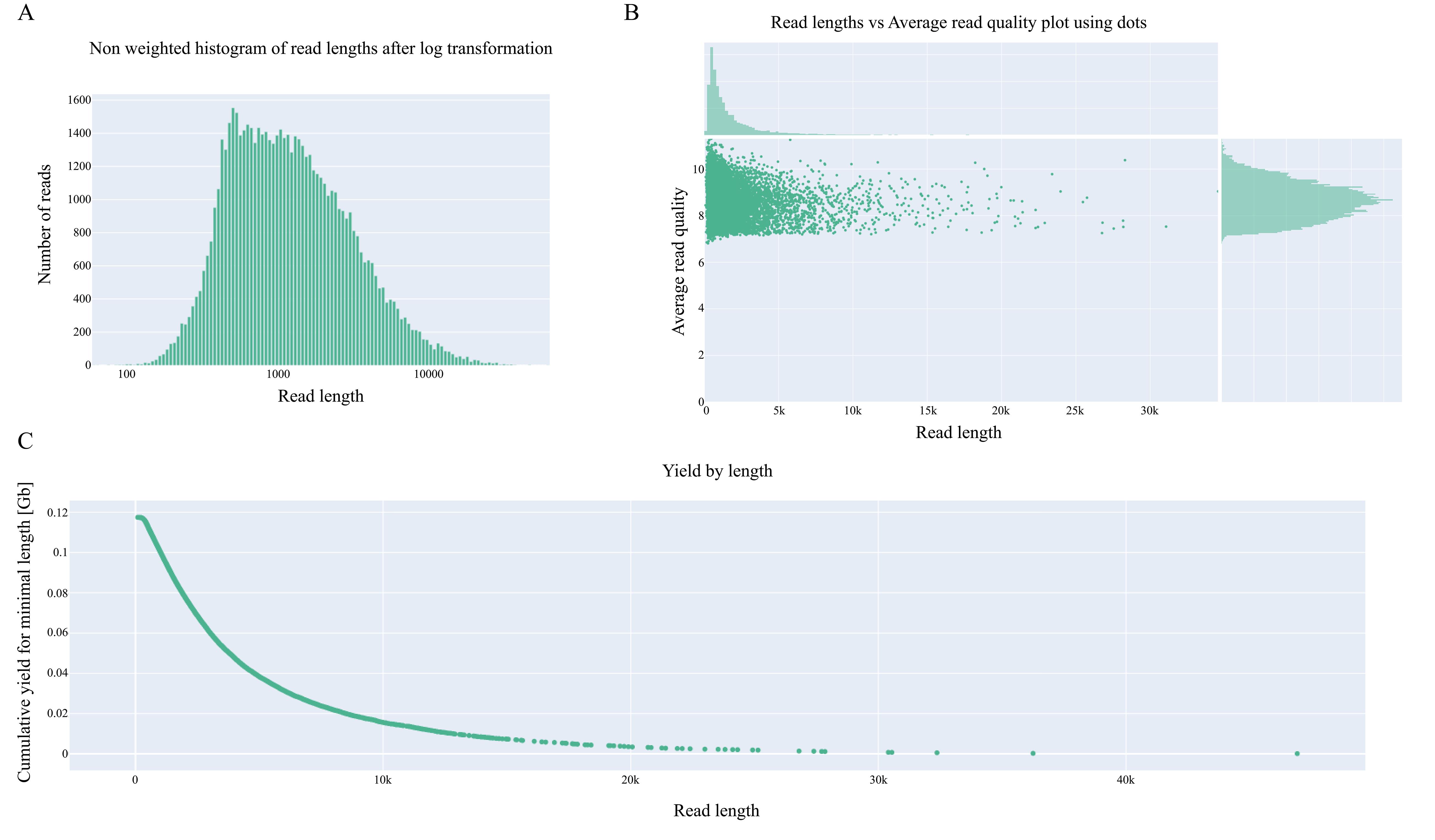
Figure 2. Visualization of NanoPlot results for the HRR2590080. (A) Non-weighted histogram of read lengths after log transformation. (B) Reads length vs. average read quality plot using dots. (C) Yield by length.
E. Trim adapters and barcodes using Porechop
Porechop is a specialized tool for Oxford Nanopore data that effectively removes adapter and barcode sequences, which is essential because residual adapters and barcodes severely impact downstream analyses by causing misalignment and false positives and interfering with structural variant detection; this trimming step is therefore critical for ensuring data integrity and analytical accuracy. Porechop requires an input FASTQ-formatted file of raw sequencing reads, and the final output is a FASTQ-formatted clean data file with adapters and barcode sequences removed.
As a first step, create a directory named “02TrimAdapters” to store all results. When trimming multiple samples, use a for loop to process all sequencing files in the RawData directory:
cd ~/eccfpwsmkdir 02TrimAdaptersls RawData/*.fastq RawData/*.fq 2>/dev/null |while read fastqdo prefix=$(echo ${fastq} |cut -d '/' -f 2 |cut -d '.' -f 1) porechop -i ${fastq} -o 02TrimAdapters/${prefix}_clean.fastq --extra_end_trim 0 --discard_middle -t 16done# Parameters Explained:# --extra_end_trim 0: No additional trimming beyond adapters# --discard_middle: Reads with middle adapters will be discarded (default: reads with middle adapters are split) (required for reads to be used with Nanopolish, this option is on by default when outputting reads into barcode bins)# -t 16: Use 16 threads for faster processingWhen using a single sample:
# Example for a single sample (e.g., HRR2590080 from PRJCA040952):porechop -i RawData/HRR2590080.fastq -o 02TrimAdapters/HRR2590080_clean.fastq --extra_end_trim 0 --discard_middle -t 16Following adapter and barcode trimming, we compared the key metrics of the raw reads and clean reads (Table S1). The results indicate a consistent improvement in the average basecall quality across most samples. It is noteworthy that sample HRR2590080, which was submitted to the repository as pre-processed clean data, showed no changes in its metrics after processing, as expected.
F. Post-adapter trimming quality assessment with NanoPlot
Following adapter and barcode removal, quality control is repeated using NanoPlot to assess the quality and characteristics of the trimmed sequencing data.
cd ~/eccfpwsmkdir 03QualityCheckls 02TrimAdapters |while read fastqdo prefix=$(echo ${fastq} |cut -d '_' -f 1) NanoPlot --fastq 02TrimAdapters/${fastq} -o 03QualityCheck/${prefix} -t 16 --plots hex dotdone# Example for a single sample (e.g., HRR2590080 from PRJCA040952):NanoPlot --fastq 02TrimAdapters/HRR2590080_clean.fastq -o 03QualityCheck/HRR2590080 -t 16 --plots hex dotThe results from this step are interpreted following the same criteria described in section D. This quality assessment serves to confirm the successful removal of adapter and barcode sequences without introducing artifacts or significant data loss. Result interpretation is the same as in section D.
G. Mapping reads to reference genomes
Following adapter and barcode trimming, the high-quality reads must be aligned to a reference genome to determine their genomic locations. Due to the distinct error profiles of long-read sequencing data compared to short-read sequencing data, aligners designed for short reads are unsuitable. We use Minimap2 for alignment, a highly efficient tool specifically optimized for long-read sequencing technologies. It provides a robust balance between mapping accuracy and computational speed. The subsequent results will be stored in the newly created 04MappingGenome directory. In this step, the input is a FASTQ-formatted clean data file with adapters and barcode sequences removed, which is aligned to the reference genome FASTA file, yielding a directly readable PAF-format alignment results file.
cd ~/eccfpws# Building reference genome index using minimap2 -d to enhances alignment efficiencyminimap2 -d Reference/GRCh38.p14.genome.fa.mmi Reference/GRCh38.p14.genome.fa# Map trimmed reads to the reference genome using minimap2mkdir 04MappingGenomels 02TrimAdapters |while read fastqdo prefix=$(echo ${fastq} |cut -d '_' -f 1) minimap2 -cx map-ont ~/eccfpws/Reference/GRCh38.p14.genome.fa.mmi 02TrimAdapters/${fastq} --secondary=no -t 16 >04MappingGenome/${prefix}.pafdone# Parameters Explained:# -cx map-ont: Optimize for Oxford Nanopore reads# --secondary=no: Filter out secondary alignments (keep only primary)# -t 16: Use 16 threads for faster processing# Example for a single sample (e.g., HRR2590080 from PRJCA040952):minimap2 -cx map-ont ~/eccfpws/Reference/GRCh38.p14.genome.fa.mmi 02TrimAdapters/HRR2590080_clean.fastq --secondary=no -t 16 >04MappingGenome/HRR2590080.pafThe alignment results demonstrate exceptionally high mapping efficiency (>95%) for the majority of samples (Table 2), confirming successful library preparation and high data quality suitable for downstream eccDNA analysis. Notably, sample SRR18143375 exhibits a markedly low mapping rate (42.76%), which may indicate substantial non-human contamination, significant genetic divergence from the reference genome, or undetected data quality issues. This outlier warrants further investigation before inclusion in subsequent analytical steps.
Table 2. Clean read alignment summary
| Clean reads | Mapped | Mapping rate (%) | Unmapped | Unmapped rate (%) | |
|---|---|---|---|---|---|
| HRR2590080 | 62787 | 61298 | 97.63 | 1489 | 2.37 |
| HRR695439 | 1233070 | 1225538 | 99.39 | 7532 | 0.61 |
| HRR695440 | 735078 | 731036 | 99.45 | 4042 | 0.55 |
| HRR695441 | 670200 | 662770 | 98.89 | 7430 | 1.11 |
| HRR695442 | 522912 | 513506 | 98.2 | 9406 | 1.8 |
| HRR695443 | 2103411 | 2007768 | 95.45 | 95643 | 4.55 |
| HRR695444 | 1264597 | 1187419 | 93.9 | 77178 | 6.1 |
| HRR695445 | 866347 | 854127 | 98.59 | 12220 | 1.41 |
| SRR18143375 | 2553645 | 1092064 | 42.76 | 1461581 | 57.24 |
| SRR18143376 | 1909357 | 1848969 | 96.84 | 60388 | 3.16 |
| SRR18143377 | 1702229 | 1628184 | 95.65 | 74045 | 4.35 |
| SRR18143378 | 4530767 | 4470407 | 98.67 | 60360 | 1.33 |
H. Identifying eccDNAs using ECCFP
ECCFP requires the sequencing FASTQ files, alignment PAF files, and the reference genome FASTA file for eccDNA identification. The tool first identifies candidate eccDNAs from individual sequencing reads and then derives accurate eccDNAs from these candidates. All ECCFP results will be saved in the 05IdentifyingEccDNA directory.
cd ~/eccfpwsmkdir 05IdentifyingEccDNAls 04MappingGenome/ |while read pafdo prefix=$(echo ${paf} |cut -d '.' -f 1) eccfp --fastq 02TrimAdapters/${prefix}_clean.fastq --paf 04MappingGenome/${paf} --reference ~/eccfpws/Reference/GRCh38.p14.genome.fa --output 05IdentifyingEccDNA/${prefix}doneUpon completion of the analysis, the 05IdentifyingEccDNA directory contains multiple subdirectories, each named after a corresponding sample and housing the respective results. Taking sample HRR2590080 as an example, its directory includes five output files: final_eccDNA.csv, consensus_sequence.fasta, variants.csv, unit.csv, and candidate_consolidated.csv. The latter two, unit.csv and candidate_consolidated.csv, serve as intermediate files: unit.csv displays candidate eccDNAs identified within individual reads, while candidate_consolidated.csv stores information related to the consolidation process from candidate to accurate eccDNAs.
Data analysis
Result interpretation
The final output comprises final_eccDNA.csv, consensus_sequence.fasta, and variants.csv. The file final_eccDNA.csv provides detailed information on accurately identified eccDNAs, including genomic position, Nfullpass representing the number of full-pass units in supporting reads, Nfragments indicating the number of genomic segments composing the eccDNA (which may originate from multiple regions), and Nreads reflecting the number of supporting reads, as well as refLength and seqLength denoting the reference genomic length and consensus sequence length, respectively (Table S2).The consensus_sequence.fasta file contains the consensus sequences for each eccDNA. Meanwhile, variants.csv documents sequence variations within eccDNAs, with columns indicating mutation coordinates, reference and alternative bases, mutant read depth and total depth at the site, mutation type, and the eccDNA harboring the variation (Table S3). In summary, this protocol provides a complete, efficient, and user-friendly workflow for eccDNA identification. As demonstrated with a single sample HRR2590080, eccDNA identification for this individual sample can be completed within approximately one hour after familiarization with the entire process (Table 3).
Table 3. Summary of runtimes for all software across the entire workflow for HRR2590080
NanoPlot (section D) | Porechop (section E) | NanoPlot (section F) | Minimap2 (section G) | ECCFP (section H) | |
|---|---|---|---|---|---|
| Runtime | 16 m 12 s | 1 m 10 s | 12 m 57 s | 1 m 54 s | 24 s |
Validation of protocol
This protocol has been validated in the following research article: Li et al. [16], iMetaOmics. 2026; e70080. DOI: 10.1002/imo2.70080. The data used in this protocol were also utilized in the aforementioned publication.
General notes and troubleshooting
General notes
1. This protocol presents the complete workflow—from quality control and alignment to eccDNA identification—with steps that can be tailored to the specific characteristics of the dataset under analysis. To facilitate first-time use and user familiarization, all datasets and the corresponding execution scripts for this protocol are made available on GitHub ( https://github.com/WSG-Lab/ECCFP_Workflow) to support reference and reproducibility.
2. Downstream analysis following eccDNA identification is not covered here, as these steps currently vary significantly depending on individual research objectives. Please conduct further exploratory analysis tailored to your specific data and goals.
3. Results may vary when using different software or dependency versions. The specific outcomes should be interpreted in the context of your actual data analysis.
Troubleshooting
1. Due to a major update in NumPy (NumPy >= 2.0.0), many built-in functions have been removed or renamed. For example, if you encounter errors such as “AttributeError: 'numpy.ndarray' object has no attribute 'ptp'” or “AttributeError: ptp was removed from the ndarray class in NumPy 2.0. Use np.ptp(arr, ...) instead.”, please install a NumPy version below 2.0. We strongly recommend using NumPy (1.26.4) for testing.
2. Throughout the workflow, minimap2 may require substantial memory, which is directly related to the size of the sequencing data input. In contrast, ECCFP has lower system memory requirements and a smaller memory footprint.
3. Low mapping rate: If the sample mapping rate is too low, it may indicate contamination or other issues with the library. Although ECCFP will still identify eccDNA from the aligned reads, the results should be used with caution.
4. The software and dependencies listed in the manuscript represent the latest versions used during the execution of the described analysis. Using different versions may affect whether the identification pipeline runs successfully. If issues are encountered, please first attempt to diagnose and resolve errors by checking the printed log messages.
5. Various issues may arise due to differences between operating systems. If you encounter problems that cannot be resolved during use, please contact the corresponding author.
GitHub page links for the above-mentioned software:
ECCFP: https://github.com/WSG-Lab/ECCFP
Porechop: https://github.com/rrwick/Porechop
Minimap2: https://github.com/lh3/minimap2
NanoPlot: https://github.com/wdecoster/NanoPlot
Pyfaidx: https://github.com/mdshw5/pyfaidx
Pyfastx: https://github.com/lmdu/pyfastx
Supplementary information
The following supporting information can be downloaded here:
1. Table S1. Read summary statistics before and after adapter and barcode trimming with Porechop.
2. Table S2. Results of eccDNA identification generated by ECCFP (final_eccDNA.csv).
3. Table S3. Results of variant information generated by ECCFP (variants.csv).
Acknowledgments
Wang Li: Conceptualization, Investigation, Writing—Original Draft; Biyuan Miao: Investigation, Writing—Original Draft; Shaogui Wan: Writing—Review & Editing, Funding acquisition, Supervision. This protocol was used in [16].
This work was supported by Key Project of Natural Science Foundation of Jiangxi Province (grant no. 20244BAB28047 and 20244BAB28030).
Competing interests
There are no conflicts of interest or competing interest.
References
- Møller, H. D., Parsons, L., Jørgensen, T. S., Botstein, D. and Regenberg, B. (2015). Extrachromosomal circular DNA is common in yeast. Proc Natl Acad Sci USA. 112(24): E3114–3122. https://doi.org/10.1073/pnas.1508825112
- Qi, K., Liu, Z., Amevor, F. K., Xu, D., Zhu, W., Li, T., Wang, Y., Wu, L., Shu, G. and Zhao, X. (2025). Emerging research insights and future perspectives on the advancement of eccDNA: a comprehensive review. Biotechnol Adv. 84: 108693. https://doi.org/10.1016/j.biotechadv.2025.108693
- Chen, S., Zhou, Z., Ye, Y., You, Z., Lv, Q., Dong, Y., Luo, J., Gong, L. and Zhu, Y. (2025). The urinary eccDNA landscape in prostate cancer reveals associations with genome instability and vital roles in cancer progression. J Adv Res. 77: 637–652. https://doi.org/10.1016/j.jare.2025.01.039
- Zeng, T., Huang, W., Cui, L., Zhu, P., Lin, Q., Zhang, W., Li, J., Deng, C., Wu, Z., Huang, Z., et al. (2022). The landscape of extrachromosomal circular DNA (eccDNA) in the normal hematopoiesis and leukemia evolution. Cell Death Discov. 8(1): 400. https://doi.org/10.1038/s41420-022-01189-w
- Yi, E., Chamorro González, R., Henssen, A. G. and Verhaak, R. G. W. (2022). Extrachromosomal DNA amplifications in cancer. Nat Rev Genet. 23(12): 760–771. https://doi.org/10.1038/s41576-022-00521-5
- Luo, J., Li, Y., Zhang, T., Xv, T., Chen, C., Li, M., Qiu, Q., Song, Y. and Wan, S. (2023). Extrachromosomal circular DNA in cancer drug resistance and its potential clinical implications. Front Oncol. 12. https://doi.org/10.3389/fonc.2022.1092705
- Liao, Z., Jiang, W., Ye, L., Li, T., Yu, X. and Liu, L. (2020). Classification of extrachromosomal circular DNA with a focus on the role of extrachromosomal DNA (ecDNA) in tumor heterogeneity and progression. Biochim Biophys Acta Rev Cancer. 1874(1): 188392. https://doi.org/10.1016/j.bbcan.2020.188392
- Turner, K. M., Deshpande, V., Beyter, D., Koga, T., Rusert, J., Lee, C., Li, B., Arden, K., Ren, B., Nathanson, D. A., et al. (2017). Extrachromosomal oncogene amplification drives tumour evolution and genetic heterogeneity. Nature. 543(7643): 122–125. https://doi.org/10.1038/nature21356
- Sihan Wu, Turner, K. M., Nguyen, N., Raviram, R., Erb, M., Santini, J., Luebeck, J., Rajkumar, U., Diao, Y., Li, B., et al. (2019). Circular ecDNA promotes accessible chromatin and high oncogene expression. Nature. 575(7784): 699–703. https://doi.org/10.1038/s41586-019-1763-5
- Møller, H. D. (2020). Circle-Seq: Isolation and Sequencing of Chromosome-Derived Circular DNA Elements in Cells. Methods Mol Biol. 2119: 165–181. https://doi.org/10.1007/978-1-0716-0323-9_15
- Wang, Y., Wang, M., Djekidel, M. N., Chen, H., Liu, D., Alt, F. W. and Zhang, Y. (2021). eccDNAs are apoptotic products with high innate immunostimulatory activity. Nature. 599(7884): 308–314. https://doi.org/10.1038/s41586-021-04009-w
- Wang, Y., Wang, M. and Zhang, Y. (2023). Purification, full-length sequencing and genomic origin mapping of eccDNA. Nat Protoc. 18(3): 683–699. https://doi.org/10.1038/s41596-022-00783-7
- Shibata, Y., Kumar, P., Layer, R., Willcox, S., Gagan, J. R., Griffith, J. D. and Dutta, A. (2012). Extrachromosomal microDNAs and chromosomal microdeletions in normal tissues. Science. 336(6077): 82–86. https://doi.org/10.1126/science.1213307
- Wanchai, V., Jenjaroenpun, P., Leangapichart, T., Arrey, G., Burnham, C. M., Tümmler, M. C., Delgado-Calle, J., Regenberg, B. and Nookaew, I. (2022). CReSIL: accurate identification of extrachromosomal circular DNA from long-read sequences. Brief Bioinform. 23(6): bbac422. https://doi.org/10.1093/bib/bbac422
- Gao, X., Liu, K., Luo, S., Tang, M., Liu, N., Jiang, C., Fang, J., Li, S., Hou, Y., Guo, C., et al. (2024). Comparative analysis of methodologies for detecting extrachromosomal circular DNA. Nat Commun. 15(1): 9208. https://doi.org/10.1038/s41467-024-53496-8
- Li, W., Miao, B., Zhang, J., Zeng, Q., Zhang, T., Wu, Z., Song, Y., Li, M., Guo, L., Luo, J., et al. (2026). ECCFP: A consecutive full pass-based bioinformatic analysis for eccDNA identification from long-read sequencing data. iMetaOmics. e70080. https://doi.org/10.1002/imo2.70080
- Li, H. (2018). Minimap2: pairwise alignment for nucleotide sequences. Bioinformatics. 34(18): 3094–3100. https://doi.org/10.1093/bioinformatics/bty191
- Li, H. (2021). New strategies to improve minimap2 alignment accuracy. Bioinformatics. 37(23): 4572–4574. https://doi.org/10.1093/bioinformatics/btab705
- De Coster, W. and Rademakers, R. (2023). NanoPack2: population-scale evaluation of long-read sequencing data. Bioinformatics. 39(5): btad311. https://doi.org/10.1093/bioinformatics/btad311
- Du, L., Liu, Q., Fan, Z., Tang, J., Zhang, X., Price, M., Yue, B. and Zhao, K. (2021). Pyfastx: a robust Python package for fast random access to sequences from plain and gzipped FASTA/Q files. Brief Bioinform. 22(4): bbaa368. https://doi.org/10.1093/bib/bbaa368
Article Information
Publication history
Received: Dec 10, 2025
Accepted: Feb 9, 2026
Available online: Feb 27, 2026
Published: Mar 20, 2026
Copyright
© 2026 The Author(s); This is an open access article under the CC BY-NC license (https://creativecommons.org/licenses/by-nc/4.0/).
How to cite
Li, W., Miao, B. and Wan, S. (2026). A Bioinformatics Workflow to Identify eccDNA Using ECCFP From Long-Read Nanopore Sequencing Data. Bio-protocol 16(6): e5636. DOI: 10.21769/BioProtoc.5636.
Category
Bioinformatics and Computational Biology
Bioinformatics
Do you have any questions about this protocol?
Post your question to gather feedback from the community. We will also invite the authors of this article to respond.