- Protocols

- Articles and Issues
- For Authors
- About
- Become a Reviewer

A Guide to Reproducible Cellulose Synthase Density and Speed Measurements in Arabidopsis thaliana
Published: Vol 16, Iss 6, Mar 20, 2026 DOI: 10.21769/BioProtoc.5634 Views: 19
Reviewed by: Felix RuhnowAnonymous reviewer(s)
Original research article
The authors used this protocol in:
Dec 2024

Protocol Collections
Comprehensive collections of detailed, peer-reviewed protocols focusing on specific topics


Abstract
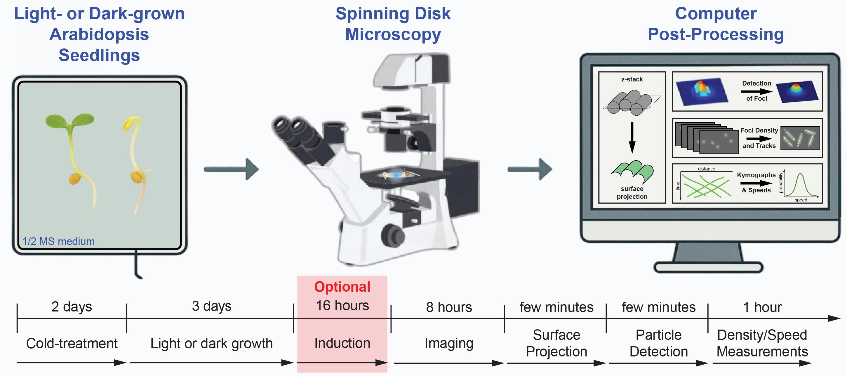
Cellulose synthase complexes (CSCs) play a central role in plant cell wall formation. Their dynamic behavior at the plasma membrane leads to the deposition of cellulose microfibrils into the apoplastic space, thereby shaping the architecture and mechanical properties of the cell wall. Although previous imaging studies have provided important insights into CSC dynamics and localization, standardized and reproducible workflows for quantitative measurements of CSC speed and density remain limited. Here, we present a reproducible live-cell imaging and analysis workflow for quantifying the speed and density of fluorescently labeled CSCs at the plasma membrane in Arabidopsis thaliana. The protocol integrates optimized spinning-disk confocal imaging, surface-based projection of z-stack recordings, automated detection of diffraction-limited CSCs foci, and kymograph-based speed measurements using freely available tools in Fiji. While selected steps, such as region of interest definition and parameter selection for spot detection or trajectory analysis, remain user-guided, these decisions are constrained to well-defined stages within an otherwise standardized pipeline, thereby reducing variability and improving reproducibility across experiments. The workflow has been validated across multiple tissues, reporter lines, genetic backgrounds, and perturbation conditions in Arabidopsis and enables robust comparative analysis of CSC dynamics. Beyond CSCs, this workflow is expected to be adaptable to other fluorescently labeled proteins that appear as diffraction-limited foci at or near the plasma membrane.
Key features
• Enables accurate CSC speed and density measurements during both primary and secondary cell wall formation using spinning-disk confocal time-lapse imaging.
• Combines surface-projection, kymograph analysis, and high-throughput particle detection to quantify CSC dynamics even in crowded or low-signal plasma membrane regions.
• Provides a standardized analysis workflow validated across multiple Arabidopsis genotypes, including inducible systems and mutant backgrounds that possess altered cell wall biosynthesis.
• Applicable to any fluorescently labeled diffraction-limited foci at or near the plasma membrane, extending the workflow beyond CSCs.
Keywords: Cellulose synthase complexes (CSC)Graphical overview
Background
Cellulose synthase A (CESA) complexes (CSCs) synthesize cellulose at the plasma membrane. In doing so, they define the mechanical properties of plant cell walls [1–4]. Their dynamic behavior, particularly their speed and density at the plasma membrane, provides direct readouts of catalytic activity, trafficking efficiency, and interactions with the cytoskeleton [5–15]. In Arabidopsis thaliana, CSCs operate in both primary cell wall (PCW) and secondary cell wall (SCW) contexts and differ in their CESA composition: PCW CSCs are heterotrimers of CESA1, CESA3, and CESA6-like isoforms, whereas SCW CSCs incorporate CESA4, CESA7, and CESA8 [2,16–22]. CSC dynamics vary with genetic background and developmental stage, and respond rapidly to environmental stimuli, making CSC motility a sensitive quantitative marker for cell wall biosynthesis [19,21,23–31].
Live-cell studies have revealed that CSCs move laterally within the plane of the plasma membrane and often track along cortical microtubules [5,7–9,22,25]. However, accurately quantifying their behavior remains challenging. Structured illumination microscopy provides high-resolution imaging of primary cell wall CSCs but is optically most reliable within shallow imaging depths near the coverslip [32]. Accordingly, imaging of cortical plasma membrane regions adjacent to the coverslip is generally advantageous for quantitative analysis. For cells or membrane domains located deeper within the tissue or further away from the coverslip, computational surface projection approaches can compensate for curvature and optical attenuation, thereby extending quantitative accessibility. Nevertheless, even under standard confocal imaging conditions, quantitative analysis is frequently complicated by background fluorescence arising from brighter and highly mobile intracellular structures such as Golgi bodies, variable signal intensities, lateral drift during time-lapse acquisition, and photobleaching. Cells with complex three-dimensional morphology, such as pavement cells, require acquisition of z-stacks that tend to highlight even more Golgi bodies, unlike hypocotyl cells that are typically imaged at a single focal plane close to the coverslip. In addition, traditional manual or semi-automated tracking approaches introduce user bias and limit throughput, particularly in crowded membrane regions where CSC trajectories overlap.
To address these limitations, we developed a reproducible workflow that integrates optimized spinning-disk confocal imaging with surface-based projection of z-stack recordings, automated diffraction-limited spot detection, and kymograph-based speed measurements. By preferentially extracting plasma-membrane surface information—for example, by applying optional surface-projection methods to suppress out-of-plane intracellular signals—and using intensity- and shape-based filtering to distinguish CSCs from Golgi-derived fluorescence, this approach robustly isolates plasma membrane–localized CSCs across diverse cell types and experimental conditions. Explicit correction for lateral drift and standardized acquisition settings further improves spatial consistency over time. Together, these elements represent a key technical advance to provide quantitative metrics suitable for comparing genotypes, treatments, and developmental stages with improved robustness and reproducibility.
This protocol therefore establishes standardized conditions for imaging, image processing, foci detection, and kymograph analysis, enabling consistent quantification of CSC speed and density across experiments and laboratories [21,28]. While the workflow does not fully eliminate user input, potential sources of user bias are restricted to a small number of well-defined and explicitly documented steps, such as region of interest (ROI) selection and parameter tuning for spot detection or projection methods. By constraining user decisions to these controlled stages and embedding them within an otherwise standardized acquisition and analysis pipeline, the protocol substantially reduces variability and improves reproducibility compared with traditional manual or ad hoc CSC-tracking approaches. Because the workflow relies on diffraction-limited spot detection and surface-based trajectory extraction rather than CSC-specific features, it is also readily applicable to other fluorescently labeled membrane-associated proteins with similar optical appearances. Although the core principles of this workflow are broadly applicable, experimental validation in the present study was performed exclusively in Arabidopsis.
Materials and reagents
Biological materials
1. SCW imaging: mNeonGreen-CESA7 (mNG-CESA7) marker in the Col-0 wild-type or the cobra-like4/irx6-2 (GK-329F09) mutant. Both lines also carried the inducible VND7-GR to induce SCW formation [33]. Request seeds from Lacey Samuels’ or Shawn Mansfield’s lab.
2. PCW imaging: GFP-CESA3 marker in the Col-0 wild type and the csi1-1/pom2-8 (SALK_136239) mutant backgrounds. Request seeds from Arun Sampathkumar’s or René Schneider’s lab.
Reagents
1. KOH (Sigma, catalog number: 484016)
2. Dexamethasone (DEX) (Sigma, catalog number: D4902-25MG)
3. Sucrose (VWR, catalog number: 27483.294)
4. MS salt including vitamins (Duchefa Biochemie, catalog number: M0222.0010)
5. MES [2-(N-morpholino)ethanesulfonic acid] (Sigma, catalog number: M8250-25g)
6. Micro-agar (Duchefa Biochemie, catalog number: M1002.1000)
7. 12.5% sodium hypochlorite (Carl Roth, catalog number: 9062.4)
8. Tween 20 (Sigma, catalog number: P1379-250ML)
9. Triton X-100 (Sigma, catalog number: X100-100ML)
10. Agarose standard (Carl Roth, catalog number: 3810.3)
11. Dimethyl sulfoxide (DMSO) (Carl Roth, catalog number: 7029.1)
12. Milli-Q water (MQ-H2O) (alternative: deionized/double-distilled H2O)
13. 1 M KOH (dissolve in MQ-H2O, store near pH meter) (Sigma, catalog number: P1767-250G)
14. 10 mM DEX (dissolve in DMSO, store 1 mL aliquots in -20 °C) (Sigma, catalog number: D4902-25MG)
Solutions
1. 1/2 MS solid medium (± 1% sucrose) (see Recipes)
2. Seed sterilization solution (see Recipes)
3. Sample holders and 1% agarose sandwiches for microscopy (see Recipes)
Recipes
1. 1/2 MS solid medium (± 1% sucrose)
| Reagent | Final concentration | Quantity or volume |
|---|---|---|
| Sucrose (optional) | 1% (w/v) | 10 g |
| MS salt (incl. vitamins) | 1/2 strength | 2.2 g |
| MES | 0.5 g | |
| 1 M KOH | to pH 5.8 | |
| MQ-H2O | top up to 800 mL |
Adjust the pH of the medium to 5.8 by carefully adding drops of 1 M KOH while stirring with a magnetic stirrer. Be careful to use the smallest drops that can be released by the glass pipette and wait a few seconds between adding additional drops to avoid overshooting the pH. After pH adjustment, bring the volume to 1,000 mL with MQ-H2O water. Transfer the solution to a bottle containing 8 g of micro-agar, mix thoroughly, and autoclave; if no agar is added, the same preparation yields standard 1/2 MS liquid medium. Store the sterilized medium in a cool, dark place (cabinet or cold room) and use within two months.
To prepare solid 1/2 MS plates, re-melt autoclaved medium in a microwave oven. To avoid boiling over, reduce microwave power to 300 W (30%). Then, allow liquefied medium to cool in a 60 °C water bath. All subsequent steps of Recipe 1 should be performed under sterile conditions in a laminar flow hood. When pharmacological treatments are required, such as the addition of selective antibiotics or DEX for induction, compounds are added at this stage to avoid heat-induced degradation. Using a sterile 50 mL Falcon tube, dispense exactly 40 or 25 mL of medium into the bottom halves of square or round plates, respectively (see Laboratory supplies). Allow plates to solidify for 15 min before covering with lids. Solidified plates are stored inverted (bottoms facing upward) in sealed plastic bags at 4 °C for up to two months.
2. Seed sterilization solution
| Reagent | Final concentration | Quantity or volume |
|---|---|---|
| 12.5% sodium hypochlorite | 1.25% | 5 mL |
| Tween 20 | n/a | 20 μL (approx. 2 drops) |
| MQ-H2O | top up to 50 mL |
Triton X-100 (same quantity) is an alternative to Tween 20.
Invert the Falcon tube several times to ensure thorough mixing; the formation of bubbles indicates proper preparation. The final solution should emit a characteristic chlorine-like odor reminiscent of public swimming pools. Store the solution at 4 °C and use within three months.
3. Sample holders and 1% agarose sandwiches for microscopy
Immediately before imaging, prepare the sample holders, have the seedlings ready for transfer, and prepare 1% agarose sandwiches to provide a stable and moist environment for the seedlings (Figure 1A–C). To prepare the agarose sandwiches, melt 1% (w/v) agarose in either MQ-H2O or liquid 1/2 MS medium. Place a 10 × 10 cm sheet of Parafilm flat on the bench and arrange individual 9 mm round cover slips on its surface (see Laboratory supplies and section B). Pipette 50–100 μL of the hot agarose onto one coverslip and place a second coverslip immediately on top, starting with the second coverslip at a 45º angle to spread the agarose evenly; slowly lower to avoid air bubbles, forming a thin, even agarose layer. Prepare additional agarose sandwiches in the same way while allowing previously assembled ones to cool and solidify.
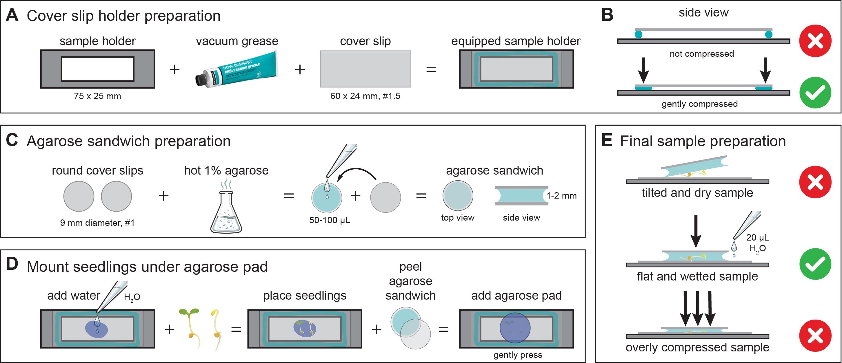
Figure 1. Preparation of correctly mounted Arabidopsis seedlings for live-cell imaging. This figure illustrates key steps for preparing stable and reproducible samples for live-cell imaging of cellulose synthase complexes. (A) Schematic showing a custom-made 75 × 25 mm microscope sample holder containing a central rectangular opening to allow optical access from below. The holder is coated with a thin layer of vacuum grease (turquoise outline), onto which a 60 × 24 mm #1.5 coverslip is mounted. Mounting seals the opening and provides a flat, stable support surface for imaging. (B) The coverslip-equipped sample holder is gently pressed to ensure firm and even adhesion of the coverslip to the holder. (C) Preparation of agarose sandwiches using two 9 mm round coverslips and molten 1% agarose. Approximately 50–100 μL of hot agarose is pipetted onto one coverslip, and the second coverslip is carefully placed on top, resulting in a solidified agarose layer of ~1–2 mm thickness between the coverslips. (D) Mounting of seedlings for imaging. Small droplets of water are placed onto the large coverslip, and seedlings are transferred onto the droplets. One coverslip is peeled off from the agarose sandwich to generate an agarose pad, which is then placed agarose-side down onto the seedlings. Residual water spreads evenly beneath the pad, forming a stable and hydrated mounting environment. (E) Common mounting errors and optimal conditions: (top) an overly dry agarose pad can tilt and mechanically stress the seedlings. (middle) This can be corrected by adding ~20 μL of water beneath the pad to achieve uniform hydration and a flat sample orientation; gentle pressure is applied only to ensure contact between the pad, liquid, and coverslip. (bottom) Excessive compression must be avoided, as it can damage both the agarose pad and the seedlings.
Laboratory supplies
1. 50 mL Falcon tubes (Roth, catalog number: AYY5.1)
2. 2 mL microcentrifuge tubes (Roth, catalog number: 5913.1)
3. 12 cm square plates (Greiner Bio-One, catalog number: 688102)
4. 9 cm round Petri dishes (Roth, catalog number: N221.2)
5. 12-well plates (Roth, catalog number: EKX6.1)
6. 9 mm round coverslips, #1 (Thermo Fisher Scientific, catalog number: 10313573)
7. 60 × 24 mm square coverslips, #1.5) (Roth, catalog number: KCY5.1)
8. Parafilm (Roth, catalog number: CNP8.1)
9. Micropore tape (1.25 cm width) (Duchefa Biochemie, catalog number: L3302)
10. ROTILAB® aluminum foil (Roth, catalog number: 2596.1)
11. Molykote high-vacuum silicone grease (Sigma, catalog number: Z273554-1EA)
Equipment
1. Fine balance (Sartorius, model: Quintix64-1S)
2. pH meter (inoLab®, model: pH 7110)
3. Magnetic stirrer (Yellow Line, model: MSH basic)
4. Orbital shaker for microcentrifuge tubes (Eppendorf, model: Thermomixer comfort)
5. Autoclave (Systec, model: VX-150)
6. Benchtop centrifuge (ROTILABO®, model: Mini centrifuge)
7. Sterile hood or clean bench (Thermo Fisher Scientific, model: MSC-Advantage)
8. Microwave oven (Sharp, model: R941)
9. Milli-Q water purification system (MERCK, model: Elix Essential 10)
10. Tilting apparatus (Lauda, model: Varioshake VS 15 R)
Software and datasets
Note: All software listed below is free to use and open source unless otherwise noted. Version numbers and release dates correspond to the versions used to develop and validate this protocol.
1. Fiji software (ImageJ2 distribution), v2.14.0 (released 2023/11/15) [34]. Free, open source (GPL license). Used for image processing, background subtraction, drift correction, and kymograph generation. Download at https://imagej.net/software/fiji/downloads
2. ThunderSTORM plugin, v1.3 (released 2014) [35]. Free, open source (GPL license). Used for spot detection and sub-pixel localization of CSC foci. Download at https://github.com/zitmen/thunderstorm
3. Smooth Manifold Projection Tool, v1.0 (released 2022). Free, open source (MIT license). Used for surface-projection of z-stack recordings to isolate plasma-membrane-localized signals. Download at https://github.com/DrReneSchneider/Smooth-Manifold-Projection-Tool
4. MultiStackReg plugin, v1.45 (released 2020) [36]. Free, open source. Used for x–y drift correction of time-lapse recordings. Download at https://github.com/miura/MultiStackRegistration
5. Bleach Correction plugin (Fiji core plugin, v1.52, released 2018) [37]. Free, open source. Used to compensate for photobleaching using histogram matching. Included with Fiji; documentation at https://imagej.net/plugins/bleach-correction
6. Velocity Measurement Tool, mod2025 version. Free, open source. Fiji macro modified by the authors to allow sequential measurements in a continuously expanding results table. The Velocity Measurement Tool (mod2025) is provided as Supplementary Dataset S1. Original references: Volker Baecker (INSERM, Montpellier RIO Imaging), J. Rietdorf (FMI Basel), A. Seitz (EMBL Heidelberg). Distributed as Supplementary Material in this manuscript.
7. FIESTA tracking software, v1.05.0005 (released 2021) [38]. Free, open source (MATLAB-based). Used as an alternative tool for automated particle tracking and high-throughput kymograph analysis. Requires a MATLAB license to run the source code; compiled macOS and Windows executables are free to use. Download at https://github.com/fiesta-tud/FIESTA/wiki
Procedure
A. Seedling growth and SCW induction (optional)
Note: This section describes the preparation, sterilization, and growth of Arabidopsis seedlings used for live-cell imaging of CSCs.
1. Seed sterilization
a. Place dry seeds on a sheet of A4 print paper and remove dust or debris by gently tapping.
b. Transfer the seeds into a 1.5 mL microcentrifuge tube.
c. Add 900 μL seed sterilization solution (see Recipes).
d. Vortex the suspension at 1,000 rpm for 10 min at room temperature.
Critical: Do not exceed 10 min; longer exposure causes seed bleaching and loss of viability.
Critical: Carry out all subsequent steps of section A under sterile conditions.
e. Briefly spin the microcentrifuge tube with a benchtop centrifuge to pellet the seeds.
f. Carefully remove the supernatant without disturbing the pellet.
g. Add 1 mL of sterile MQ-H2O, resuspend the seeds gently, and allow them to settle.
h. Remove supernatant, resuspend seeds in 1 mL of sterile MQ-H2O, and repeat four times, allowing settling between washes.
i. Store the sterilized seeds at 4 °C for 2–3 days to stratify.
Pause point: Stratified seeds can be stored for up to 7 days to enhance germination efficiency, but extended cold storage may cause seeds to germinate prematurely in the tube.
2. Seed plating and germination
a. Prepare square or round plates containing solid 1/2 MS medium (with or without 1% sucrose).
b. Position sterilized seeds on the surface of the medium using an autoclaved pipette tip or toothpick.
c. Seal plates with several rounds of micropore tape so that no gaps remain and the plate cover is fixed properly.
d. Wrap plates in two layers of aluminum foil to induce etiolated growth.
e. Incubate the aluminum foil–wrapped plates in a vertical orientation in a climate-controlled growth cabinet at 22 °C (day) and 18 °C (night) for 3 days.
Notes:
1. Exposure of plated seeds to full light for at least 4 h before wrapping them with aluminum foil enhances germination efficiency.
2. Alternatively, plate sterilized seeds (from step A1h) directly on solid 1/2 MS medium and perform cold treatment at 4 °C for 2–3 days (up to 7 days) on the plates.
3. (Optional) DEX induction of SCW formation in VND7-GR plant lines
a. Prepare approximately 10 mL of 10 μM DEX in liquid 1/2 MS solution by diluting the DEX stock 1:1,000.
b. For liquid induction: Transfer 3-day-old etiolated seedlings into 1–2 mL of 10 μM DEX solution in a sterile 12-well plate, ensuring that the entire seedling (including hypocotyl and cotyledons) is fully submerged. Incubate for 16–24 h at room temperature in complete darkness; 16 h corresponds to the onset of SCW formation, and 24 h corresponds to late SCW formation and early programmed cell death.
Critical: Avoid shaking the seedlings, as vigorous motion can damage fragile tissues, especially the apical hook. Use a tilting apparatus (see Equipment) at 20 rpm instead of an orbital shaker to gently agitate the medium.
Note: When seedlings are maintained in complete darkness during induction, induced and non-induced seedlings cannot be distinguished based on their appearance.
c. Alternatively, transfer seedlings onto fresh 1/2 MS plates supplemented with 10 μM DEX using sterile toothpicks.
B. Live-cell imaging and preparation of seedling samples
Note: This section describes the preparation of seedlings for microscopy and the acquisition parameters for spinning-disk confocal imaging during CSC analysis. For imaging sessions lasting up to 24 h, sample preparation can be performed under non-sterile conditions. For longer imaging sessions, we recommend preparing samples under sterile conditions to minimize contamination.
1. Sample holder and mounting of seedlings
a. Mount a #1.5 coverslip (60 × 25 mm) onto a metal slide holder (75 × 25 mm) using a thin layer of Molykote high-vacuum silicone grease (Figure 1A). The custom-made slide holder contains a central rectangular opening (50 × 20 mm) for optical access.
b. Carefully press the coverslip onto the sample holder to ensure firm and even adhesion between the coverslip and the slide holder (Figure 1B).
c. Prepare 1% agarose sandwiches for microscopy (see Recipes and Figure 1C) and store them in a Petri dish with moist filter paper to prevent drying.
d. Distribute 25 μL of sterile MQ-H2O or liquid 1/2 MS medium by pipetting small droplets onto the coverslip surface (Figure 1D).
e. Gently transfer up to three seedlings onto the coverslip with forceps or toothpicks. The previously deposited droplets help to stick the seedling to the coverslip.
f. Peel off the round coverslip from the agarose sandwich and carefully place the agarose side onto the seedlings on the coverslip to immobilize the sample.
Critical: Ensure even contact between the seedlings and the coverslip surface by gently adjusting the agarose sandwich (e.g., using a toothpick) to maintain a stable focal plane (Figure 1E). Excessive pressure should be avoided, as imaging cells in close contact with the coverslip can, in principle, introduce mechanical compression artifacts. To minimize such effects, seedlings should be immobilized using a thin agarose layer without applying external force. Add sufficient sterile water to the agarose layer to maintain a moist mounting environment and visually inspect cell morphology to exclude regions showing signs of deformation.
2. (Optional) Identification of induced seedlings following light exposure during induction
a. When SCW induction is performed under light conditions, identify seedlings with successful SCW induction by the presence of 1) an unopened apical hook and 2) yellowish cotyledons.
Note: Under continuous dark conditions, successful SCW induction cannot be reliably inferred from external seedling morphology and should be assessed microscopically.
b. Inspect epidermal cotyledon and upper hypocotyl cells for ectopic banded SCW patterns (Figure 2).
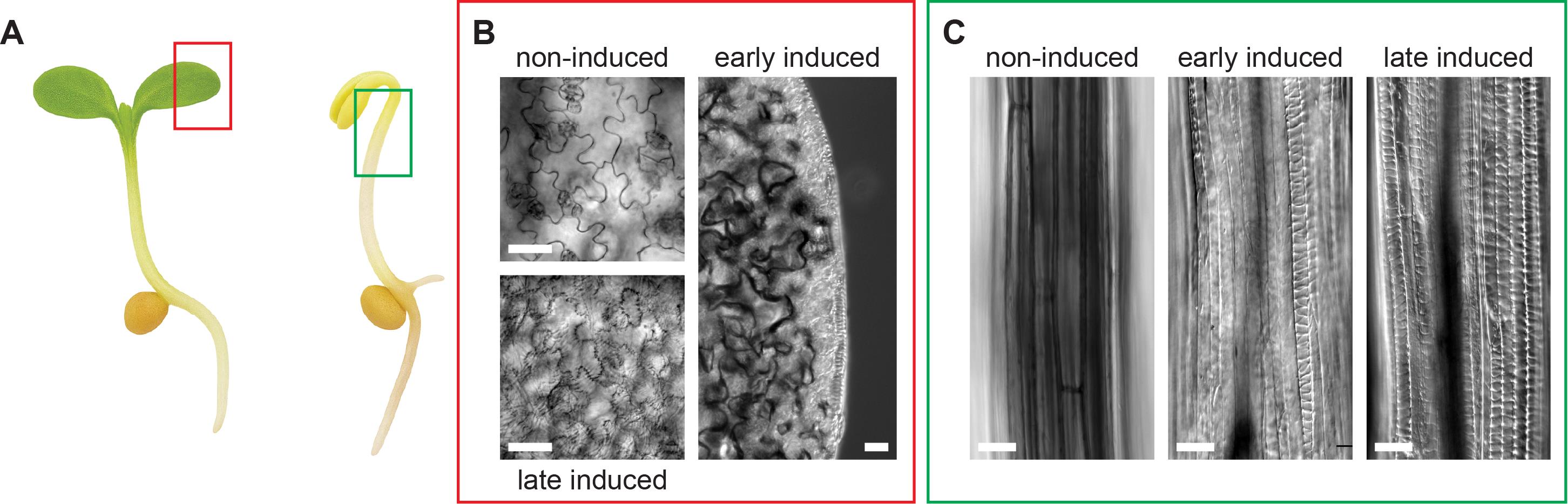
Figure 2. Identification of successful secondary cell wall (SCW) induction in Arabidopsis seedlings. (A) Schematic representation of light- and dark-grown Arabidopsis seedlings, highlighting the tissue regions typically analyzed following SCW induction. Red and green boxes indicate the cotyledons and upper hypocotyl, respectively. (B) Cotyledon epidermal pavement cells at different stages of SCW induction (red box in A). Top left, non-induced pavement cells. Right, early induction stage, with cells at the cotyledon margin responding first. Bottom left, fully induced cotyledon epidermis showing transdifferentiated pavement cells with characteristic patterned SCWs. Scale bar: 20 μm. (C) Hypocotyl epidermal cells at different stages of SCW induction (green box in A). Left, non-induced hypocotyl cells. Middle, early induction stage, with individual cells responding first. Right, fully transdifferentiated hypocotyl cells exhibiting patterned SCWs. Scale bar: 50 μm.
Critical: Prioritize cells in direct contact with the glass coverslip for long-term imaging, as their focal plane remains stable over time.
3. Microscope setup
a. Use a spinning-disk confocal microscope equipped with either 1) 100× oil-immersion objective (NA 1.4), 2) 63× water-immersion objective (NA 1.2), or 3) other high-magnification objectives with comparable image-forming properties.
b. Excite fluorescent CESA reporters using a 488 or 491 nm laser line appropriate for GFP- or mNG-tagged constructs.
c. Collect green fluorescence emission in the 500–550 nm window.
d. Use either an EMCCD or sCMOS camera.
Note: Keep laser power, exposure time, and gain identical for all samples to ensure accurate comparison.
4. (Optional) Time-lapse acquisition (XYT)
Note: While single-slice (XY) recordings may, in principle, suffice for CSC density measurements, time-lapse (XYT) and z-stack (XYZ) recordings often improve data quantity and quality, and statistical robustness (Figure 3A–C). Moreover, because CSC speed quantification requires temporal information, time-lapse acquisition or time-lapse z-stack (XYZT) recordings are generally advisable (Figure 3D).
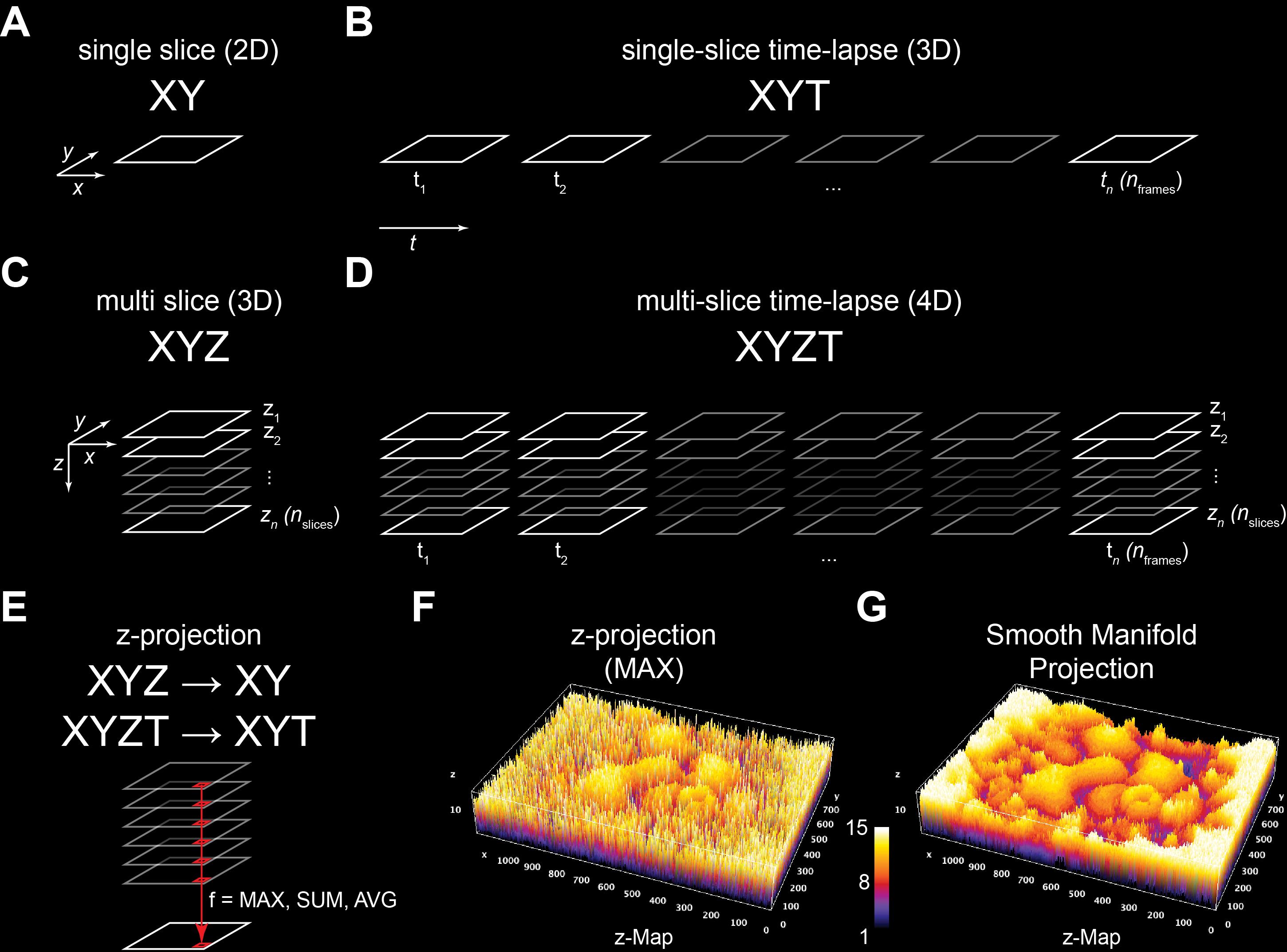
Figure 3. Naming conventions for microscopy recording modalities. (A) Single-slice (XY) recording acquired at a single focal plane and time point. (B) Single-slice time-lapse (XYT) recording acquired at one focal plane over multiple time points. (C) Multi-slice (XYZ) recording consisting of a z-stack acquired across multiple focal planes at a single time point. (D) Multi-slice time-lapse (XYZT) recording combining z-stack acquisition with time-lapse imaging across multiple time points. (E) A z-projection creates a new XY image from volumetric XYZ data by performing maximum (MAX), sum (SUM), or average (AVG) operations within each column of pixels along the z-direction. (F) A z-map corresponding to a conventional z-projection (MIP). For MIPs, neighboring pixels in the projected image may originate from different z-slices, resulting in a highly discontinuous z-map and ambiguous spatial relationships. (G) In contrast, smooth manifold projection identifies a continuous surface—ideally corresponding to the cell surface—from which pixel intensities are sampled, thereby preserving local spatial relationships in the projected image. Note the improved delineation of cell surfaces compared to the MIP z-map shown in (F). Color bars indicate the z-position in the original stack from where each projected pixel intensity was obtained.
Note: On inverted microscopes, z-stacks are typically acquired from the coverslip upward; this figure is not intended to imply a specific acquisition direction.
a. Record 5–15 min time-lapse sequences of CSCs in epidermal cells.
Note: When available, record a second fluorescence channel in parallel to visualize additional cellular structures, such as microtubules.
5. (Optional) Estimating optimal time intervals for time-lapse recordings
a. Calculate the optimal time interval between frames ΔTopt using the following formula:
where Dpixel is the camera pixel size (in nm) at the applied magnification, and VCSC is the predicted CSC speed (in nm/min). Example: For Dpixel = 100 nm and VCSC = 200 nm/min, set ΔTopt = 30 s.
b. Set frame intervals to the calculated optimum or alternatively between 5 and 60 s.
Note: For optimal imaging of CSCs, adjust the focal plane to the region of the plasma membrane in direct contact with the glass coverslip, providing a flat and stable imaging surface. Use the in-built focus stabilization (auto-focus) of most commercial instruments to maintain this plane throughout acquisition.
6. (Optional) Acquisition of z-stacks
a. When larger imaging volumes or entire cell outlines are desired, acquire XYZ or XYZT stacks of 5–20 slices (nslices) with a 0.3 μm step size (Figure 3C, D).
b. Ensure the z-range spans from the apoplastic space into deeper cytoplasmic regions.
Critical: The limited photostability of fluorescent reporters necessitates balancing laser exposure with the need for 3D information, especially during XYZT acquisition.
Critical: Keep laser power and acquisition settings (e.g., exposure time, gain) constant across all samples.
Critical: Confocal imaging introduces heat into the biological specimen, which influences CSC behavior and density. To minimize temperature-induced artifacts, maintain comparable imaging durations and acquisition schemes across all samples.
Note: In most commercial instruments, a focus stabilization (auto-focus) option can also be used to stabilize and maintain the reference plane for z-stacks.
C. Image processing steps and optional z-projection for XYZ and XYZT recordings
Note: This section describes the generation and processing of XY and XYT datasets for subsequent CSC speed and density analyses. When working with multi-slice datasets (XYZ or XYZT), z-projection is performed as the first processing step. Other processing operations, such as lateral drift or photobleaching correction, and background subtraction, are applied after z-projection.
1. Generation of XY and XYT stacks from XYZ and XYZT recordings
Notes:
1. When CSCs are imaged as multi-slice datasets (XYZ or XYZT), a z-projection must be applied to generate single-slice XY or XYT stacks suitable for downstream analysis. The purpose of the z-projection is to collapse fluorescence signals originating from different focal planes onto a single XY image (Figure 3E).
2. A commonly used approach is maximum-intensity projection (MIP), which generates an XY image from volumetric data by retaining, for each x–y pixel position, only the highest-intensity value along the z-axis. Although MIPs are widely used, they frequently fail to accurately represent the plasma membrane–localized CSC population. This limitation arises because bright intracellular structures (e.g., Golgi stacks or cytoplasmic strands) often dominate the projection and obscure the typically weaker CSC signals. In addition, MIPs treat individual pixel columns independently, thereby disrupting spatial relationships between neighboring pixels and complicating biological interpretation (Figure 3F).
a. Apply a z-projection to the XYZ or XYZT dataset using Image → Stacks → Z Project in Fiji. Select an appropriate projection method from the drop-down menu; maximum (MAX), sum (SUM), or average (AVG) projections are most commonly used.
b. Visually inspect the resulting projection. If plasma membrane–localized CSC trajectories are continuous and clearly distinguishable from intracellular fluorescence, proceed with the selected MAX, SUM, or AVG projection for subsequent analysis. If internal structures (e.g., Golgi bodies) obscure CSC trajectories at the plasma membrane, apply a smooth manifold projection to generate a surface-optimized projection.
Notes:
1. The smooth manifold projection algorithm operates on a z-map that records, for each pixel, the z-slice from where the maximal intensity originates (Figure 3F, G). The rugged MIP z-map (Figure 3F) is smoothed by fitting a two-dimensional envelope with user-defined stiffness, analogous to draping a tablecloth over uneven objects (Figure 3G). Fluorescence intensities corresponding to this inferred surface—ideally approximating the cell surface—are then extracted from the original XYZ or XYZT dataset, preserving local spatial relationships between neighboring pixels.
2. When inspecting projections, users should also examine the corresponding z-map generated by the projection method. A suitable projection is characterized by a smooth and spatially continuous z-map in which much of the cellular surface is consistently identified and largely free of abrupt depth jumps or discontinuities. Highly fragmented or irregular z-maps typically indicate contamination by out-of-plane intracellular signals and are less suitable for quantitative CSC analysis (see Figure 3F, G for examples).
c. Apply the Smooth Manifold Projection tool listed in the Software and datasets section. The algorithm is implemented as a MATLAB-based script that is freely available online, and a Fiji-compatible version providing equivalent functionality is also available. For assistance with the Fiji implementation, contact the Schneider Lab.
2. Drift correction: If lateral drift is observed, apply the MultiStackReg tool (Plugins → Registration → MultiStackReg) using the Translation transform to correct x–y drift.
Critical: This plugin offers a versatile set of registration options suitable for most types of drift encountered in biological microscopy. Be careful using the Rigid body or Affine transforms, as they may introduce distortions.
3. Bleach correction: If photobleaching occurs during time-lapse imaging, apply the Bleach Correction plugin using the Match Histogram option. In the latest Fiji versions, this tool can be found under Image → Adjust → Bleach Correct.
Note: This approach equalizes frame histograms while preserving relative intensity differences.
4. Background subtraction
a. Enhance the visibility of CSC signals by applying Process → Subtract Background in Fiji using a rolling-ball radius of 5–15 pixels (Figure 4A, B).
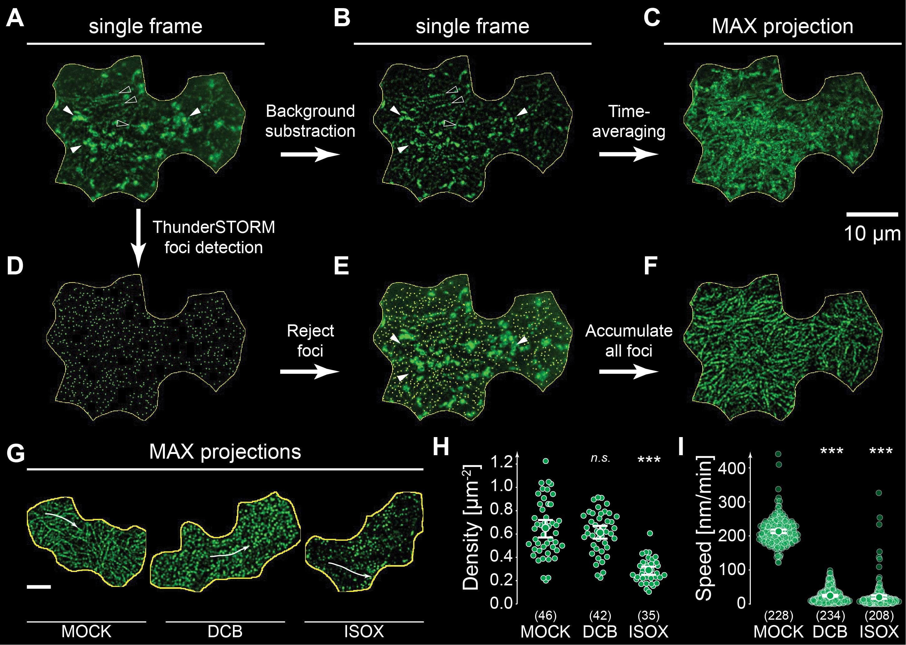
Figure 4. Image processing and automated detection of cellulose synthase complex (CSC) foci using ThunderSTORM. (A) Smooth manifold–projected single frame of a cotyledon epidermal cell two days after germination, showing plasma membrane–localized CSCs (empty arrowheads) and bright, mobile Golgi bodies (filled arrowheads). (B) Rolling-ball background subtraction suppresses bright internal Golgi signals while preserving CSC tracks. (C) Time-averaging by maximum-intensity projection (MIP) of background-subtracted frames; overlapping Golgi signals obscure fine CSC trajectories, limiting suitability for speed analysis. (D) ThunderSTORM spot detection: each fluorescent focus is approximated by a two-dimensional Gaussian intensity distribution and displayed on a reconstructed “Gaussian-only” image, rendering rolling-ball background subtraction obsolete (see panels A and B). (E) Intensity-based filtering (offset > 1 count; 5–60 nm localization uncertainty; 50–500 nm sigma; intensity <500,000 counts) rejects bright Golgi signals and enhances CSC detection accuracy. (F) Average shifted histogram (ASH) image or time-accumulated reconstruction (e.g., via MIP) of all ThunderSTORM-detected foci reveals membrane trajectories, including those in dim regions. (G–I) Example analysis of CSC responses to cellulose-synthesis inhibitors in 2-day-old cotyledon epidermal cells. (G) Time-accumulated ThunderSTORM reconstructions in mock-treated cells and in cells treated for 4 h with 2,6-dichlorobenzonitrile (DCB) or isoxaben (ISOX). (H) CSC density quantification: DCB maintains wild-type CSC abundance at the plasma membrane (≈0.6 CSC·μm-2), whereas ISOX induces CSC internalization, reducing density by ~50%. (I) CSC speed quantification: both DCB and ISOX markedly reduce CSC velocities, indicating inhibition of cellulose synthase activity. CSC speeds are reported in nm/min for consistency with the literature (1 nm/min ≈ 0.0167 nm/s). Statistical comparisons use Welch’s unpaired t-test (***p < 0.001). Scale bars: 10 μm (all panels). Panels A–F shown in this figure are adapted from Schneider et al. [21] and are reproduced under the terms of the Creative Commons Attribution 4.0 International License (CC BY 4.0).
b. Assess the effect of background subtraction by generating a time-averaged image (XYT → XY) using Image → Stacks → Z Project.
c. Inspect the resulting image visually to verify that linear CSC trajectories at the plasma membrane are preserved, while fluorescence from intracellular structures such as Golgi stacks is effectively suppressed.
Note: If background fluorescence remains dominant, faint CSC trajectories may be obscured and become difficult to detect (Figure 4C). In such cases, consider using the ThunderSTORM Fiji plugin (step D1a) for spot detection as an alternative strategy.
D. Quantification of CSC density at the plasma membrane
Note: This section outlines high-throughput detection of CSC foci using the ThunderSTORM Fiji plugin (Figure 4D–F). ThunderSTORM, originally developed for stochastic optical reconstruction microscopy (STORM) applications, identifies diffraction-limited fluorescence peaks and reconstructs an image containing idealized Gaussian representations of these foci across all time points of an XYT recording. The total number of detected foci, normalized to the analyzed area and number of frames, provides an estimate of CSC density.
1. Spot detection with ThunderSTORM
a. Load the processed XYT stack into Fiji.
Note: While single-slice (XY) recordings may suffice for CSC density measurements, XYT datasets are used here by default to improve statistical robustness. CSC density calculations treat detections in individual frames as independent observations and therefore reflect the instantaneous surface occupancy of CSCs within a defined membrane area rather than the number of unique CSC trajectories. Averaging detections across multiple frames reduces the influence of transient fluctuations and enables robust relative density comparisons between conditions when identical acquisition and analysis parameters are applied.
b. Use the Freehand Selection tool to outline a ROI containing well-illuminated plasma membrane areas.
c. Open Plugins → ThunderSTORM → Run Analysis.
d. In Camera Setup, enter the camera pixel size (in nm), set Photoelectrons per A/D count to 1, and adjust Base level according to the camera’s minimum background count.
e. Select Wavelet filter (B-spline) and set order = 3 and scale = 2.
f. Choose Local Maximum detection with std(Wave.F1) threshold and 8-neighbourhood connectivity.
g. Select PSF: Integrated Gaussian to allow sub-pixel localization accuracy, set fitting radius = 3 pixels, initial sigma = 1.6 pixels, and choose the Weighted Least Squares fitting method.
h. For visualization, choose Averaged Shifted Histogram and set Magnification = 1 to maintain the original XYT stack dimensions.
i. Start the analysis by clicking OK.
2. ThunderSTORM output
a. ThunderSTORM generates 1) a table of detected foci, listing each spot with parameters including x–y coordinates, peak intensity, sigma, offset, background noise, and localization uncertainty, 2) an overlay of the detected spots on the original stack for visual inspection, and 3) a reconstructed Gaussian-only image termed “averaged shifted histogram” (ASH) (Figure 4D–F).
Note: Save the reconstructed ASH for subsequent speed analysis and CSC trajectory identification (section E, Figure 4F).
b. Apply the following filters to remove non-CSC structures (Figure 4E):
i. offset > 1 count
ii. 5 nm < localization uncertainty < 60 nm
iii. 50 nm < sigma < 500 nm
iv. intensity < 500,000 counts (adjust this threshold as needed for your imaging conditions)
3. Density calculation
a. Filter the results by selecting Apply.
b. Export the filtered table and sum over all individual foci (ni) that were detected across all frames (nframes).
c. Compute CSC density (σCSC) as follows:
where nfoci = total number of detected foci, AROI = area of the ROI (in μm2), and nframes = number of time points.
Notes:
1. The area of the analyzed region (AROI) is obtained in Fiji by selecting the ROI using the freehand selection or polygon selection tools and recording the enclosed area via Analyze → Measure. The measured area is reported in μm2, provided the image is calibrated.
2. Because CSC density estimates depend on the choice of the analyzed membrane area, ROI selection represents a controlled, user-defined step in the workflow. To minimize variability, ROIs should encompass continuous, well-illuminated plasma-membrane regions and avoid areas dominated by internal fluorescence or low signal-to-noise ratios. When applied consistently across samples, this approach yields robust relative density comparisons between conditions. Alternative strategies, such as Voronoi-based area estimation from ThunderSTORM-derived point clouds, can in principle be used to derive local density measures but are not implemented here and fall outside the scope of this protocol.
Pause point: The original and filtered ThunderSTORM results should be stored and reused for subsequent speed analysis (section E, Figure 4F).
E. Quantification of CSC speed
Note: This section describes manual kymograph-based CSC speed measurements in Fiji and defines sampling requirements (Figure 5). Kymographs generated from surface-projected XYT recordings enable reliable extraction of CSC trajectories along user-defined paths, providing a robust alternative to automated tracking in complex datasets. The workflow and the minimum number of CSCs needed for statistically robust speed estimates are outlined here.
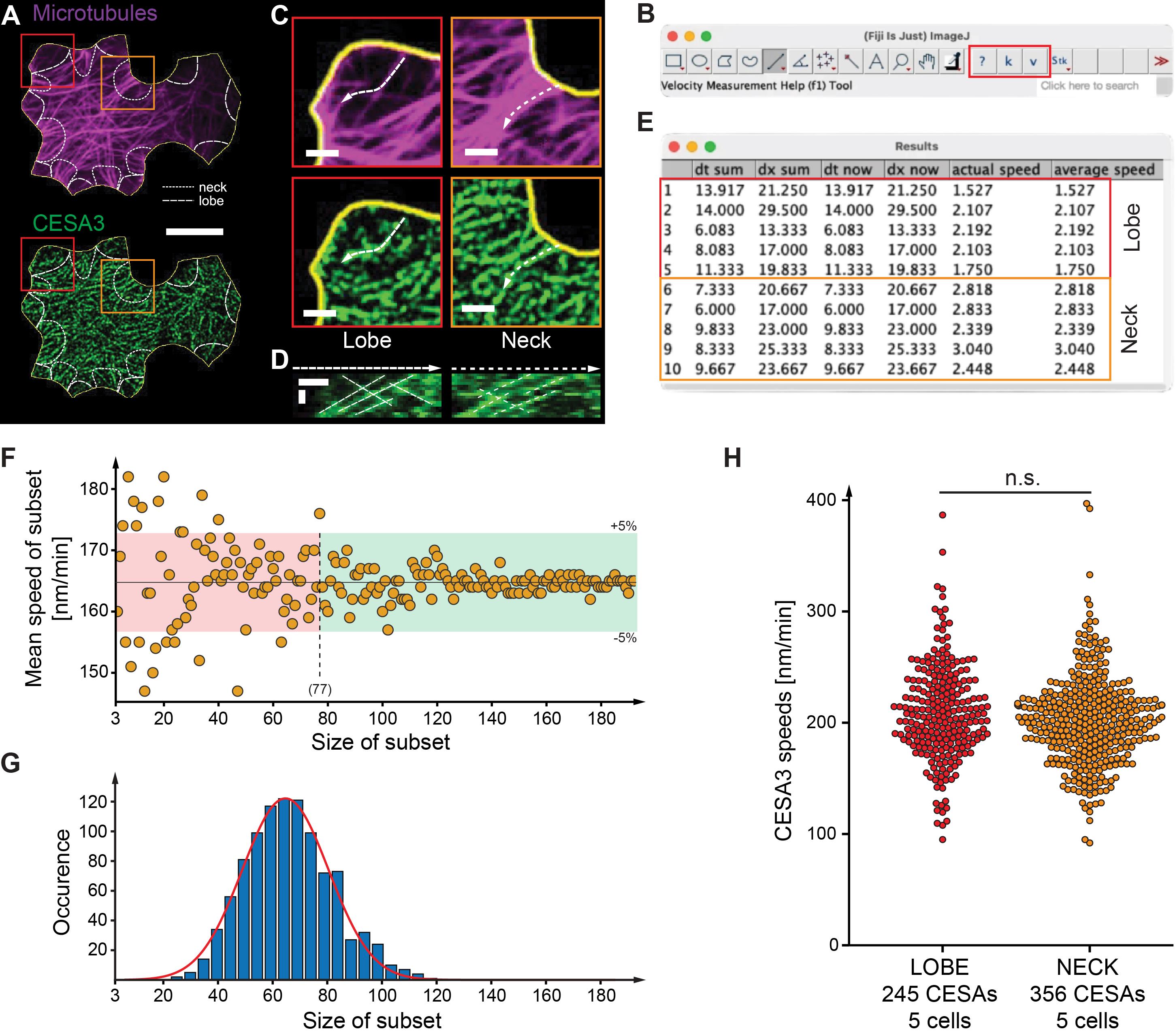
Figure 5. Manual kymograph-based quantification of cellulose synthase complex (CSC) speed using Fiji. (A) Averaged shifted histogram (ASH) images of mCherry-TUA5-labeled microtubules (magenta, top) and GFP-CESA3-labeled CSCs (green, bottom) in a single 2-day-old cotyledon pavement cell (yellow outline). Lobe and neck regions are outlined by dashed and dotted lines, respectively. Scale bar = 10 μm. (B) The modified Velocity Measurement Tool adds three buttons to the Fiji toolbar: ? (help), k (generate kymograph), and v (measure trajectory slope = speed). (C) Enlarged ASH image regions (boxes in panel A) showing lobes (red) and necks (orange) for microtubules (top) and CSCs (bottom). Scale bar = 2 μm. (D) Kymographs generated from the dashed and dotted ROIs in panel C using the k function. Slanted lines represent moving CSCs. Scale bars = 1 μm (spatial) and 5 min (temporal). (E) Example velocity measurements of individual CSC trajectories in panel D using the v function. (F) Subsampling analysis for one cell (192 CSC trajectories total). Mean CSC speed was recalculated for increasing subset sizes; from ~77 trajectories onward, all subset means fell within the 95% confidence interval of the full dataset. (G) Bootstrapping (1,000 iterations) revealed that subsets including 64 ± 1 CSC trajectory are sufficient on average to obtain stable mean speed estimates. (H) Application of optimized subset sizes to compare CSC speeds in neck and lobe regions. Across five cells (356 CSCs in necks = 71 trajectories per cell; 245 CSCs in lobes = 49 trajectories per cell), no significant difference in CSC speed was detected. CSC speeds are reported in nm/min for consistency with the literature (1 nm/min ≈ 0.0167 nm/s). Panels A, C, and D shown in this figure are adapted from Schneider et al. [21] and are reproduced under the terms of the Creative Commons Attribution 4.0 International License (CC BY 4.0).
1. Open the z-projected XYT stack and the ASH image in Fiji (Figure 5A).
2. Install the Velocity Measurement Tool (VMT, mod2025) via Plugins → Macros → Install. Installation adds three buttons to the Fiji toolbar (Figure 5B): ? opens the help file, k generates a kymograph from a user-defined line ROI, and v measures the slope of a selected line within the kymograph.
3. Use the Straight Line or Segmented Line tool to draw ROIs along visible CSC trajectories in the ASH image. Alternatively, generate a time-projection of the XYT stack (e.g., MIP or SUM) to obtain an image for trajectory selection.
4. Transfer each ROI to the XYT stack using Edit → Selection → Restore Selection.
5. Press k to generate the kymograph (Figure 5C, D).
Note: If a second channel (e.g., microtubules) is available, its signal can be used to guide ROI placement. In this case, define ROIs from a SUM, AVG, or MIP projection of the microtubule XYT recording rather than from the ASH image (Figure 5A, C, D).
6. Measuring CSC speeds
a. In the kymograph, identify slanted trajectories representing moving CSCs.
Note: Stationary foci appear as vertical lines. Shallower (more horizontal) slopes correspond to moving CSC.
b. Using the Straight Line or Segmented Line tool, trace each slanted trajectory.
c. Press v to calculate the speed.
Note: For each selected trajectory, the results table reports the duration of the measured segment (Δt) and the spatial distance covered during that duration (Δx), given in pixel-per-frame values. The table also provides instantaneous (“now”) or, for segmented lines, average (“sum”) CSC speeds (Figure 5E).
d. Convert pixel-per-frame speeds to physical units using the following formula:
where the final conversion factor translates speeds from nm/s to nm/min.
e. (Alternative) FIESTA (open-source, MATLAB-based, graphical user interface) offers automated tracking and high-throughput kymograph analysis [39]. Originally developed for single-molecule in vitro assays, it also performs well in crowded in vivo datasets.
7. Determining minimum sample size
a. For one cell, measure ≥200 CSC speeds to build a reference dataset.
b. Arrange the measured CSC speeds in random order and subsample this dataset using increasing sample sizes ranging from 3 to the total N.
c. Identify the smallest subset for which most mean speeds repeatedly fall within the 95% CI of the full dataset.
d. Under typical imaging conditions, 40–75 CSC tracks per cell are sufficient (Figure 5F–H).
Notes:
1. Avoid oversampling; restricting measurements to a reasonable sample size improves throughput without compromising accuracy.
2. Alternative velocity-estimation strategies based on automated frame-to-frame pairing of detected foci, such as nearest-neighbor assignment or particle image velocimetry (PIV)-like approaches, can in principle be applied to ThunderSTORM output to derive CSC velocities across large datasets. These methods reduce manual input and benefit from averaging over large numbers of measurements, thereby mitigating individual tracking errors. However, such approaches require careful handling of foci appearance, disappearance, and trajectory crossing, particularly in crowded membrane regions. In this protocol, we therefore focus on kymograph-based analysis, which provides direct visual validation of individual CSC trajectories and remains robust under conditions of variable signal quality. Users seeking higher-throughput alternatives may adapt PIV- or pairing-based approaches as appropriate for their datasets.
8. User-dependent steps and reproducibility considerations: While this workflow provides standardized acquisition and analysis steps for CSC quantification, several stages remain inherently user-guided. These include selection of the analyzed membrane region, choice of projection method (e.g., MIP vs. surface-based projection), parameter tuning for automated foci detection, and selection of representative CSC trajectories for kymograph-based analysis. Among these, ROI definition and projection choice typically contribute the largest variability between datasets, whereas spot detection and kymograph analysis are comparatively robust once appropriate parameters are established. To improve inter-user reproducibility, we recommend applying consistent ROI selection criteria, documenting all analysis parameters, and validating projection quality and CSC trajectories by visual inspection. Where possible, reproducibility can further be assessed by parallel analysis of shared example datasets or by independent reanalysis using identical parameter sets.
Validation of protocol
We validated this protocol using multiple Arabidopsis cell types, imaging conditions, and analysis tools to demonstrate its robustness, reproducibility, and suitability for quantitative comparisons of CSC behavior [21,28]. This analysis encompassed distinct tissues, reporter lines, mutant backgrounds, and pharmacological perturbations. While the protocol has not been experimentally validated in other plant species, its reliance on generic imaging and analysis principles suggests that it can be readily adapted to comparable systems.
1. Validation of CSC density measurements: We evaluated the ThunderSTORM-based detection pipeline using seedlings expressing GFP-CESA3 or mNG-CESA7 (representative results shown in Figure 4G–I). In cotyledon epidermal cells, ThunderSTORM reliably detected diffraction-limited CSC foci under both control conditions and after inhibitor treatments. Treatment with the cellulose synthesis inhibitor isoxaben reduced plasma-membrane CSC density by approximately 50%, whereas DCB treatment maintained wild-type densities. These responses match established phenotypes and confirm that the workflow accurately reproduces known biological outcomes [21,40,41]. The filtering criteria for offset, sigma, localization uncertainty, and intensity consistently removed Golgi-derived signals while retaining CSC tracks across independent experiments. Across three biological replicates per treatment, coefficient-of-variation values remained within 8%–15%, demonstrating that the density measurements produced by this pipeline are stable and reproducible.
2. Validation of CSC speed measurements: We validated the manual kymograph-based speed measurements using independent datasets and multiple cells (Figure 5). In one representative cell, 192 CSC trajectories were quantified, and sampling speeds in random order showed that a subset of ≥77 trajectories reproduced a mean speed within 95% confidence intervals of the mean obtained for all 192 trajectories (Figure 5F). Bootstrapping across 1,000 random iterations further suggested that, on average, 64 trajectories are sufficient to obtain stable mean velocity estimates under our imaging conditions (Figure 5G). Using this optimized sampling strategy, we compared CSC speeds between lobe and neck regions of cotyledon pavement cells and found no measurable difference between the two regions across five biological replicates (356 CSCs in necks; 245 CSCs in lobes; Figure 5H). Mean CSC speeds were 202 ± 40 nm/min in necks and 207 ± 43 nm/min in lobes. These analyses demonstrate that the protocol yields reproducible CSC speed measurements, even when comparing structurally distinct subcellular regions.
3. Validation across biological contexts and imaging systems: This pipeline performs reliably across the major developmental stages in which CSC dynamics are typically examined. It supports quantification of GFP-CESA3 speed and density in expanding pavement cells during PCW formation, as well as analysis of mNG-CESA7 behavior in wild-type and irx6-2 mutants during SCW formation in inducible VND7 systems (hypocotyl epidermis cells). The workflow also consistently detects the expected CSC responses to drug perturbations, including the contrasting effects of isoxaben and DCB, and remains robust in crowded membrane regions with high CSC density and/or frequent Golgi motion. Reproducible measurements were obtained using both 100× oil immersion and 63× water immersion objectives and with either EMCCD or sCMOS detectors (data not shown), demonstrating the method’s stability across imaging platforms.
4. Validation through application in published research: Parts of this protocol have already been applied and validated in multiple peer-reviewed studies. Xue et al. [28] used the workflow to quantify mNG-CESA7 speeds and densities in wild-type and irx6-2 backgrounds and to assess how COBRA-LIKE4 influences CSC mobility. Schneider et al. [21] applied the same core pipeline to measure GFP-CESA3 speeds and densities during developmental progression, cytoskeletal perturbation, and mechanical stimulation in pavement cells. In addition, the core principles of sample preparation, image preprocessing, and density quantification were implemented in Schneider et al. [42] to quantify the density of GFP-labeled GCP3 nucleation complexes along cortical microtubules in secondary cell wall–forming cells. Across these studies, the workflow consistently reproduced expected biological responses and resolved subtle mutant phenotypes, demonstrating robustness across independent labs, imaging setups, and experimental conditions.
Xue et al. [28] used this workflow to quantify mNG-CESA7 particle speeds (Figure 2 and Supplementary Figure S3) and densities in wild-type and irx6-2 (mutant of COBRA-LIKE4) backgrounds (Supplementary Figure S4) and to analyze mNG-CESA7 foci sizes and fluorescence intensities (Supplementary Figure S5). Schneider et al. [21] applied this protocol to assess GFP-CESA3 particle speeds and densities during cotyledon development (Figure 1 and Supplementary Figures S2–4), under oryzalin treatment, in csi1-1/pom2-8 (mutants of CELLULOSE SYNTHASE INTERACTING1) (Figure 2 and Supplementary Figure S5), and during mechanical perturbations such as tissue ablation and compression (Figure 5 and Supplementary Figures S7–8).
General notes and troubleshooting
General notes
1. Ensure consistency in imaging conditions across samples. Laser power, exposure time, camera gain, and objective choice strongly influence CSC signal quality and apparent density. For comparative experiments, maintain identical acquisition settings and durations across genotypes, treatments, and replicates (see General note 4).
2. The protocol is broadly applicable to other diffraction-limited, plasma membrane–localized proteins. Although optimized for CSCs, the workflow also performs well for any fluorescently labeled foci that appear within or near plasma membranes. Adaptation typically requires only changing fluorescent channels and spot-detection thresholds.
3. Surface projection improves analysis in tissues with curved or uneven cell surfaces. The Smooth Manifold Projection Tool (suitable alternatives include methods by Shihavuddin et al. [43] and Erguvan et al. [44]) is particularly useful in thick tissues or curved cells, where standard MIPs mix cytoplasmic and membrane signals [43–45]. In samples with naturally flat membranes, such as epidermal cells pressed against the coverslip, a simple MIP is often sufficient.
4. Biological variability in CSC density and speed is expected. CSC behavior varies with developmental stage, cell type, light environment, and cell wall status [21,27]. When performing comparative studies, use age-matched seedlings and analyze cells from equivalent positions to minimize confounding variation.
5. ThunderSTORM settings may require optimization across imaging systems. Camera noise levels, pixel sizes, and optical magnifications influence peak-detection thresholds. The recommended filtering parameters work robustly for the imaging systems tested but may require adjustments for other microscopes.
6. Kymograph-based speed measurements assume directed CSC motion along the plasma membrane. This method is most accurate when CSC trajectories are linear and well-defined. In conditions where CSC motility becomes irregular or highly curved (e.g., after cytoskeletal disruption), automated tracking tools such as FIESTA may complement manual kymographs [7,46].
7. Crowded membrane regions require careful ROI selection. High densities of CSCs, Golgi bodies, or background structures can increase false-positive detection or obscure CSC trajectories. Select ROIs with high signal-to-noise ratios and avoid regions containing excessive internal fluorescence.
8. The recommended sample size for CSC speed measurements applies broadly but may vary with signal quality. Subsampling and bootstrapping indicate that ~40–75 trajectories per cell provide stable velocity estimates under typical conditions. In noisier datasets or lower-expression lines, more trajectories per cell may be needed.
9. This workflow is compatible with both PCW and SCW systems. It has been validated in expanding pavement cells, in hypocotyl and root epidermis, in inducible VND7 systems, and in mutant backgrounds that show altered CSC trafficking or cellulose synthesis. When applying the protocol to other tissues, verify that CSCs remain within the focal plane long enough for reliable measurements.
10. Training in Fiji and familiarity with basic image analysis greatly improve reproducibility. Users unfamiliar with kymograph analysis, spot detection, or the use and/or design of macros should review the Fiji user guides (https://imagej.net/learn/user-guides) before applying the protocol. This ensures a correct interpretation of projections, ROIs, and speed readouts.
Troubleshooting
Problem 1: CSCs are difficult to see or appear dim and non-motile.
Possible causes: Incorrect focal plane, selected cell is too far from the glass coverslip, weak reporter expression, or CSC trajectories hidden within background noise.
Solutions: Focus strictly on plasma-membrane regions that are near or in direct contact with the glass coverslip; if necessary, gently press onto the agar sandwich so that epidermal cells adhere closer to the glass surface. Use seedlings 2–3 days after germination, when PCW CSC density is highest [21], and select reporter lines with strong expression. To reveal weak CSC motility in noisy datasets, acquire a longer time-lapse with a larger frame interval (e.g., 1 min) and replay the movie at a high frame rate. This often makes subtle, noise-obscured CSC trajectories visible.
Problem 2: Bright Golgi bodies obscure CSC signals and create false positives in ThunderSTORM.
Possible causes: Incomplete background subtraction, strong internal fluorescence, mechanical stress causing CSC internalization, or imaging older cells with abundant Golgi.
Solutions: Apply rolling-ball background subtraction (5–15 pixel radius) or use Smooth Manifold Projection if Golgi signals still dominate. Ensure seedlings are not mechanically stressed and image slightly younger tissue if Golgi abundance is high. When CSC tracks are present but masked by noise, use temporal averaging (e.g., walking-average projections) to improve visibility. In ThunderSTORM, reduce false positives by filtering out the brightest and widest spots (high intensity, large sigma) before calculating densities.
Problem 3: ThunderSTORM detects too many spurious peaks.
Possible causes: Single-pixel noise, low signal-to-noise ratio, overly permissive peak-detection thresholds, or incorrect baseline settings during analysis.
Solutions: Confirm that pixel size and baseline values are correctly entered in the ThunderSTORM Camera Setup panel. Apply a smoothing step (e.g., average or median filter) before running ThunderSTORM to reduce isolated single-pixel noise. If necessary, tighten post-detection filters by narrowing the acceptable localization-uncertainty or sigma ranges.
Problem 4: ThunderSTORM detects too few CSCs.
Possible causes: ROI too small, overly stringent filters, low signal-to-noise ratio, or bleaching.
Solutions: Expand the ROI to include all membrane regions with visible tracks. Relax filtering thresholds incrementally (e.g., allow slightly larger sigma values). Reduce laser power to limit bleaching but increase exposure time moderately to improve signal-to-noise ratio. Confirm that membrane contact with the coverslip is optimal.
Problem 5: Lateral drift in the time-lapse leads to distorted CSC tracks or incorrect speed measurements.
Possible causes: Seedling movement, mechanical instability, or thermal drift.
Solutions: Apply MultiStackReg (in translation mode) before any downstream analysis. Verify that the seedling is immobilized (agarose sandwich recommended). Allow the sample to equilibrate thermally for 5–10 min before starting acquisitions.
Problem 6: Bleach correction distorts relative fluorescence intensity over time.
Possible causes: Mismatched bleaching profile or inappropriate histogram matching.
Solutions: Confirm that Match Histogram is appropriate for your dataset; if bleaching is severe or nonlinear, avoid correction altogether and instead optimize laser power and exposure to minimize bleaching at the acquisition level.
Supplementary information
The following supporting information accompanies this protocol and can be downloaded here:
1. Dataset S1. Velocity Measurement Tool (mod2025): Fiji macro file containing the modified Velocity Measurement Tool used for generating kymographs and extracting CSC velocities as described in section E. This version supports sequential measurements appended to a continuously growing results table and includes minor interface improvements for reproducible CSC speed analysis.
Acknowledgments
Conceptualization, R.S.; Investigation, J.Y.X. and R.S.; Writing—original draft, R.S.; Writing—review and editing, J.Y.X., S.D.M., A.L.S., A.S., and R.S.; Funding acquisition, S.D.M., A.L.S., A.S., and R.S.; Supervision, S.D.M., A.L.S., A.S., and R.S. This work was supported by Deutsche Forschungsgemeinschaft (DFG; grant no. 453188536 to R.S. and project no. 512328399 to R.S. and A.S.). Additional support was provided by the German Federal Ministry of Education and Research (BMBF; SHAPENET project 031L0177B to A.S.) and by Natural Sciences and Engineering Research Council of Canada (NSERC) Discovery Grants to A.L.S. (RGPIN-2025-05870) and S.D.M. (RGPIN-2024-04385). We acknowledge foundational work on which components of this protocol rely, including Fiji (Schindelin et al. [34]), the ThunderSTORM plugin (Ovesný et al. [35]), the MultiStackReg plugin (Thévenaz et al. [36]), the Velocity Measurement Tool developed by Volker Baecker (INSERM, Montpellier RIO Imaging), J. Rietdorf (FMI Basel), and A. Seitz (EMBL Heidelberg), and the FIESTA tracking software (Ruhnow et al. [38]). These contributions enabled the development and refinement of the workflow presented in this manuscript.
Competing interests
The authors declare no conflicts of interest.
References
- Polko, J. K. and Kieber, J. J. (2019). The Regulation of Cellulose Biosynthesis in Plants. Plant Cell. 31(2): 282–296. https://doi.org/10.1105/tpc.18.00760
- Wilson, T. H., Kumar, M. and Turner, S. R. (2021). The molecular basis of plant cellulose synthase complex organisation and assembly. Biochem Soc Trans. 49(1): 379–391. https://doi.org/10.1042/bst20200697
- Pedersen, G. B., Blaschek, L., Frandsen, K. E., Noack, L. C. and Persson, S. (2023). Cellulose synthesis in land plants. Mol Plant. 16(1): 206–231. https://doi.org/10.1016/j.molp.2022.12.015
- Cosgrove, D. J. (2023). Structure and growth of plant cell walls. Nat Rev Mol Cell Biol. 25(5): 340–358. https://doi.org/10.1038/s41580-023-00691-y
- Paredez, A. R., Somerville, C. R. and Ehrhardt, D. W. (2006). Visualization of Cellulose Synthase Demonstrates Functional Association with Microtubules. Science. 312(5779): 1491–1495. https://doi.org/10.1126/science.1126551
- Gutierrez, R., Lindeboom, J. J., Paredez, A. R., Emons, A. M. C. and Ehrhardt, D. W. (2009). Arabidopsis cortical microtubules position cellulose synthase delivery to the plasma membrane and interact with cellulose synthase trafficking compartments. Nat Cell Biol. 11(7): 797–806. https://doi.org/10.1038/ncb1886
- Chan, J. and Coen, E. (2020). Interaction between Autonomous and Microtubule Guidance Systems Controls Cellulose Synthase Trajectories. Curr Biol. 30(5): 941–947.e2. https://doi.org/10.1016/j.cub.2019.12.066
- Bringmann, M., Li, E., Sampathkumar, A., Kocabek, T., Hauser, M. T. and Persson, S. (2012). POM-POM2/CELLULOSE SYNTHASE INTERACTING1 Is Essential for the Functional Association of Cellulose Synthase and Microtubules in Arabidopsis. Plant Cell. 24(1): 163–177. https://doi.org/10.1105/tpc.111.093575
- Gu, Y., Kaplinsky, N., Bringmann, M., Cobb, A., Carroll, A., Sampathkumar, A., Baskin, T. I., Persson, S. and Somerville, C. R. (2010). Identification of a cellulose synthase-associated protein required for cellulose biosynthesis. Proc Natl Acad Sci USA. 107(29): 12866–12871. https://doi.org/10.1073/pnas.1007092107
- Li, S., Lei, L., Somerville, C. R. and Gu, Y. (2011). Cellulose synthase interactive protein 1 (CSI1) links microtubules and cellulose synthase complexes. Proc Natl Acad Sci USA. 109(1): 185–190. https://doi.org/10.1073/pnas.1118560109
- Chen, S., Ehrhardt, D. W. and Somerville, C. R. (2010). Mutations of cellulose synthase (CESA1) phosphorylation sites modulate anisotropic cell expansion and bidirectional mobility of cellulose synthase. Proc Natl Acad Sci USA. 107(40): 17188–17193. https://doi.org/10.1073/pnas.1012348107
- Kumar, M., Wightman, R., Atanassov, I., Gupta, A., Hurst, C. H., Hemsley, P. A. and Turner, S. (2016). S-Acylation of the cellulose synthase complex is essential for its plasma membrane localization. Science. 353(6295): 166–169. https://doi.org/10.1126/science.aaf4009
- Zhu, Y. and McFarlane, H. E. (2022). Regulation of cellulose synthesis via exocytosis and endocytosis. Curr Opin Plant Biol. 69: 102273. https://doi.org/10.1016/j.pbi.2022.102273
- Zhu, X., Li, S., Pan, S., Xin, X. and Gu, Y. (2018). CSI1, PATROL1, and exocyst complex cooperate in delivery of cellulose synthase complexes to the plasma membrane. Proc Natl Acad Sci USA. 115(15): e1800182115. https://doi.org/10.1073/pnas.1800182115
- Vellosillo, T., Dinneny, J. R., Somerville, C. R. and Ehrhardt, D. W. (2021). TRANVIA (TVA) facilitates cellulose synthase trafficking and delivery to the plasma membrane. Proc Natl Acad Sci USA. 118(30): e2021790118. https://doi.org/10.1073/pnas.2021790118
- Persson, S., Paredez, A., Carroll, A., Palsdottir, H., Doblin, M., Poindexter, P., Khitrov, N., Auer, M. and Somerville, C. R. (2007). Genetic evidence for three unique components in primary cell-wall cellulose synthase complexes in Arabidopsis. Proc Natl Acad Sci USA. 104(39): 15566–15571. https://doi.org/10.1073/pnas.0706592104
- Desprez, T., Juraniec, M., Crowell, E. F., Jouy, H., Pochylova, Z., Parcy, F., Höfte, H., Gonneau, M. and Vernhettes, S. (2007). Organization of cellulose synthase complexes involved in primary cell wall synthesis in Arabidopsis thaliana. Proc Natl Acad Sci USA. 104(39): 15572–15577. https://doi.org/10.1073/pnas.0706569104
- Taylor, N. G., Howells, R. M., Huttly, A. K., Vickers, K. and Turner, S. R. (2003). Interactions among three distinct CesA proteins essential for cellulose synthesis. Proc Natl Acad Sci USA. 100(3): 1450–1455. https://doi.org/10.1073/pnas.0337628100
- Li, S., Bashline, L., Zheng, Y., Xin, X., Huang, S., Kong, Z., Kim, S. H., Cosgrove, D. J. and Gu, Y. (2016). Cellulose synthase complexes act in a concerted fashion to synthesize highly aggregated cellulose in secondary cell walls of plants. Proc Natl Acad Sci USA. 113(40): 11348–11353. https://doi.org/10.1073/pnas.1613273113
- Xu, H., Giannetti, A., Sugiyama, Y., Zheng, W., Schneider, R., Watanabe, Y., Oda, Y. and Persson, S. (2022). Secondary cell wall patterning—connecting the dots, pits and helices. Open Biol. 12(5): e210208. https://doi.org/10.1098/rsob.210208
- Schneider, R., Ehrhardt, D. W., Meyerowitz, E. M. and Sampathkumar, A. (2022). Tethering of cellulose synthase to microtubules dampens mechano-induced cytoskeletal organization in Arabidopsis pavement cells. Nat Plants. 8(9): 1064–1073. https://doi.org/10.1038/s41477-022-01218-7
- Schneider, R., Tang, L., Lampugnani, E. R., Barkwill, S., Lathe, R., Zhang, Y., McFarlane, H. E., Pesquet, E., Niittyla, T., Mansfield, S. D., et al. (2017). Two Complementary Mechanisms Underpin Cell Wall Patterning during Xylem Vessel Development. Plant Cell. 29(10): 2433–2449. https://doi.org/10.1105/tpc.17.00309
- Sampathkumar, A., Gutierrez, R., McFarlane, H. E., Bringmann, M., Lindeboom, J., Emons, A. M., Samuels, L., Ketelaar, T., Ehrhardt, D. W., Persson, S., et al. (2013). Patterning and Lifetime of Plasma Membrane-Localized Cellulose Synthase Is Dependent on Actin Organization in Arabidopsis Interphase Cells. Plant Physiol. 162(2): 675–688. https://doi.org/10.1104/pp.113.215277
- Liu, Z., Schneider, R., Kesten, C., Zhang, Y., Somssich, M., Zhang, Y., Fernie, A. R. and Persson, S. (2016). Cellulose-Microtubule Uncoupling Proteins Prevent Lateral Displacement of Microtubules during Cellulose Synthesis in Arabidopsis. Dev Cell. 38(3): 305–315. https://doi.org/10.1016/j.devcel.2016.06.032
- Liu, L., Wang, T., Bai, Y., Yan, P., Dai, L., Du, P., Persson, S. and Zhang, Y. (2023). Actomyosin and CSI1/POM2 cooperate to deliver cellulose synthase from Golgi to cortical microtubules in Arabidopsis. Nat Commun. 14(1): 7442. https://doi.org/10.1038/s41467-023-43325-9
- Watanabe, Y., Meents, M. J., McDonnell, L. M., Barkwill, S., Sampathkumar, A., Cartwright, H. N., Demura, T., Ehrhardt, D. W., Samuels, A., Mansfield, S. D., et al. (2015). Visualization of cellulose synthases in Arabidopsis secondary cell walls. Science. 350(6257): 198–203. https://doi.org/10.1126/science.aac7446
- Watanabe, Y., Schneider, R., Barkwill, S., Gonzales-Vigil, E., Hill, J. L., Samuels, A. L., Persson, S. and Mansfield, S. D. (2018). Cellulose synthase complexes display distinct dynamic behaviors during xylem transdifferentiation. Proc Natl Acad Sci USA. 115(27): e1802113115. https://doi.org/10.1073/pnas.1802113115
- Xue, J. Y., McNair, G., Watanabe, Y., Kaplen, M. V., Guevara-Rozo, S., Schuetz, M., Schneider, R., Mansfield, S. D. and Samuels, A. L. (2024). COBRA-LIKE4 modulates cellulose synthase velocity and facilitates cellulose deposition in the secondary cell wall. Plant Physiol. 196(4): 2531–48. https://doi.org/10.1093/plphys/kiae469
- Zhang, Y., Nikolovski, N., Sorieul, M., Vellosillo, T., McFarlane, H. E., Dupree, R., Kesten, C., Schneider, R., Driemeier, C., Lathe, R., et al. (2016). Golgi-localized STELLO proteins regulate the assembly and trafficking of cellulose synthase complexes in Arabidopsis. Nat Commun. 7(1): e1038/ncomms11656. https://doi.org/10.1038/ncomms11656
- Endler, A., Kesten, C., Schneider, R., Zhang, Y., Ivakov, A., Froehlich, A., Funke, N. and Persson, S. (2015). A Mechanism for Sustained Cellulose Synthesis during Salt Stress. Cell. 162(6): 1353–1364. https://doi.org/10.1016/j.cell.2015.08.028
- Sánchez-Rodríguez, C., Ketelaar, K., Schneider, R., Villalobos, J. A., Somerville, C. R., Persson, S. and Wallace, I. S. (2017). BRASSINOSTEROID INSENSITIVE2 negatively regulates cellulose synthesis in Arabidopsis by phosphorylating cellulose synthase 1. Proc Natl Acad Sci USA. 114(13): 3533–3538. https://doi.org/10.1073/pnas.1615005114
- Duncombe, S. G., Chethan, S. G. and Anderson, C. T. (2021). Super-resolution imaging illuminates new dynamic behaviors of cellulose synthase. Plant Cell. 34(1): 273–286. https://doi.org/10.1093/plcell/koab227
- Yamaguchi, M., Goué, N., Igarashi, H., Ohtani, M., Nakano, Y., Mortimer, J. C., Nishikubo, N., Kubo, M., Katayama, Y., Kakegawa, K., et al. (2010). VASCULAR-RELATED NAC-DOMAIN6 and VASCULAR-RELATED NAC-DOMAIN7 Effectively Induce Transdifferentiation into Xylem Vessel Elements under Control of an Induction System. Plant Physiol. 153(3): 906–914. https://doi.org/10.1104/pp.110.154013
- Schindelin, J., Arganda-Carreras, I., Frise, E., Kaynig, V., Longair, M., Pietzsch, T., Preibisch, S., Rueden, C., Saalfeld, S., Schmid, B., et al. (2012). Fiji: an open-source platform for biological-image analysis. Nat Methods. 9(7): 676–682. https://doi.org/10.1038/nmeth.2019
- Ovesný, M., Křížek, P., Borkovec, J., Švindrych, Z. and Hagen, G. M. (2014). ThunderSTORM: a comprehensive ImageJ plug-in for PALM and STORM data analysis and super-resolution imaging. Bioinformatics. 30(16): 2389–2390. https://doi.org/10.1093/bioinformatics/btu202
- Thévenaz, P., Ruttimann, U. and Unser, M. (1998). A pyramid approach to subpixel registration based on intensity. IEEE Trans Image Process. 7(1): 27–41. https://doi.org/10.1109/83.650848
- Miura, K. (2020). Bleach correction ImageJ plugin for compensating the photobleaching of time-lapse sequences. F1000Research. 9: 1494. https://doi.org/10.12688/f1000research.27171.1
- Ruhnow, F., Zwicker, D. and Diez, S. (2011). Tracking Single Particles and Elongated Filaments with Nanometer Precision. Biophys J. 100(11): 2820–2828. https://doi.org/10.1016/j.bpj.2011.04.023
- Schneider, R., Sampathkumar, A. and Persson, S. (2019). Quantification of Cytoskeletal Dynamics in Time‐Lapse Recordings. Curr Protoc plant Biol. 4(2): e20091. https://doi.org/10.1002/cppb.20091
- DeBolt, S., Gutierrez, R., Ehrhardt, D. W. and Somerville, C. (2007). Nonmotile Cellulose Synthase Subunits Repeatedly Accumulate within Localized Regions at the Plasma Membrane in Arabidopsis Hypocotyl Cells following 2,6-Dichlorobenzonitrile Treatment. Plant Physiol. 145(2): 334–338. https://doi.org/10.1104/pp.107.104703
- Liu, D., Zehfroosh, N., Hancock, B. L., Hines, K., Fang, W., Kilfoil, M., Learned-Miller, E., Sanguinet, K. A., Goldner, L. S., Baskin, T. I., et al. (2017). Imaging cellulose synthase motility during primary cell wall synthesis in the grass Brachypodium distachyon. Sci Rep. 7(1): 15111. https://doi.org/10.1038/s41598-017-14988-4
- Schneider, R., Klooster, K.V., Picard, K. L., van der Gucht, J., Demura, T., Janson, M., Sampathkumar, A., Deinum, E.E., Ketelaar, T., Persson, S. (2021). Long-term single-cell imaging and simulations of microtubules reveal principles behind wall patterning during proto-xylem development. Nat Commun. 12(1): 669. https://doi.org/10.1038/s41467-021-20894-1
- Shihavuddin, A., Basu, S., Rexhepaj, E., Delestro, F., Menezes, N., Sigoillot, S. M., Del Nery, E., Selimi, F., Spassky, N., Genovesio, A., et al. (2017). Smooth 2D manifold extraction from 3D image stack. Nat Commun. 8(1): 15554. https://doi.org/10.1038/ncomms15554
- Erguvan, Ã., Louveaux, M., Hamant, O. and Verger, S. (2019). ImageJ SurfCut: a user-friendly pipeline for high-throughput extraction of cell contours from 3D image stacks. BMC Biol. 17(1): 38. https://doi.org/10.1186/s12915-019-0657-1
- Eng, R. C., Schneider, R., Matz, T. W., Carter, R., Ehrhardt, D. W., Jönsson, H., Nikoloski, Z. and Sampathkumar, A. (2021). KATANIN and CLASP function at different spatial scales to mediate microtubule response to mechanical stress in Arabidopsis cotyledons. Curr Biol. 31(15): 3262–3274.e6. https://doi.org/10.1016/j.cub.2021.05.019
- Jacobs, B., Schneider, R., Molenaar, J., Filion, L. and Deinum, E. E. (2022). Microtubule nucleation complex behavior is critical for cortical array homogeneity and xylem wall patterning. Proc Natl Acad Sci USA. 119(50): e2203900119. https://doi.org/10.1073/pnas.2203900119
Article Information
Publication history
Received: Dec 17, 2025
Accepted: Feb 5, 2026
Available online: Feb 26, 2026
Published: Mar 20, 2026
Copyright
© 2026 The Author(s); This is an open access article under the CC BY-NC license (https://creativecommons.org/licenses/by-nc/4.0/).
How to cite
Readers should cite both the Bio-protocol article and the original research article where this protocol was used:
- Xue, J. Y., Mansfield, S. D., Samuels, A. L., Sampathkumar, A. and Schneider, R. (2026). A Guide to Reproducible Cellulose Synthase Density and Speed Measurements in Arabidopsis thaliana. Bio-protocol 16(6): e5634. DOI: 10.21769/BioProtoc.5634.
- Xue, J. Y., McNair, G., Watanabe, Y., Kaplen, M. V., Guevara-Rozo, S., Schuetz, M., Schneider, R., Mansfield, S. D. and Samuels, A. L. (2024). COBRA-LIKE4 modulates cellulose synthase velocity and facilitates cellulose deposition in the secondary cell wall. Plant Physiol. 196(4): 2531–48. https://doi.org/10.1093/plphys/kiae469
Category
Plant Science > Plant cell biology > Cell imaging
Cell Biology > Cell imaging
Do you have any questions about this protocol?
Post your question to gather feedback from the community. We will also invite the authors of this article to respond.