- Protocols

- Articles and Issues
- For Authors
- About
- Become a Reviewer

Machine Learning-Assisted Quantification of Organelle Abundance
(§Technical contact: A.J.Long@soton.ac.uk) Published: Vol 16, Iss 5, Mar 5, 2026 DOI: 10.21769/BioProtoc.5626 Views: 82
Reviewed by: Akira KarasawaAnonymous reviewer(s)
Original research article
The authors used this protocol in:
Sep 2025

Protocol Collections
Comprehensive collections of detailed, peer-reviewed protocols focusing on specific topics


Abstract
Organelle abundance is a key microscopic readout of organelle formation and, in many cases, function. Quantification of organelle abundance using confocal microscopy requires estimating their area based on the fluorescence intensity of compartment-specific markers. This analysis usually depends on a user-defined intensity threshold to distinguish organelle regions from the surrounding cytoplasm, which introduces potential bias and variability. To address this issue, we present a machine learning–assisted algorithm that allows for the quantification of organelle density using the open-source Fiji platform and WEKA segmentation. Our method enables the automated quantification of organelle number, area, and density by learning from training data. This standardizes threshold selection and minimizes user intervention. We demonstrate the utility of this approach for both membrane and non-membrane organelles, such as peroxisomes, lipid droplets, and stress granules, in human cells and whole fish samples.
Key features
• The organelle abundance algorithm is an automated, open-source, Fiji-based tool that extracts organelle number and area and calculates abundance based on a single marker.
• The macro measures the average intensity of all the segmented areas and quantifies their area.
• The algorithm is applicable to cellular compartments, including membrane-bound and membrane-less organelles.
• The training is performed on a sample dataset, enabling the algorithm to be applied to all images obtained with the same imaging parameters.
Keywords: OrganelleGraphical overview
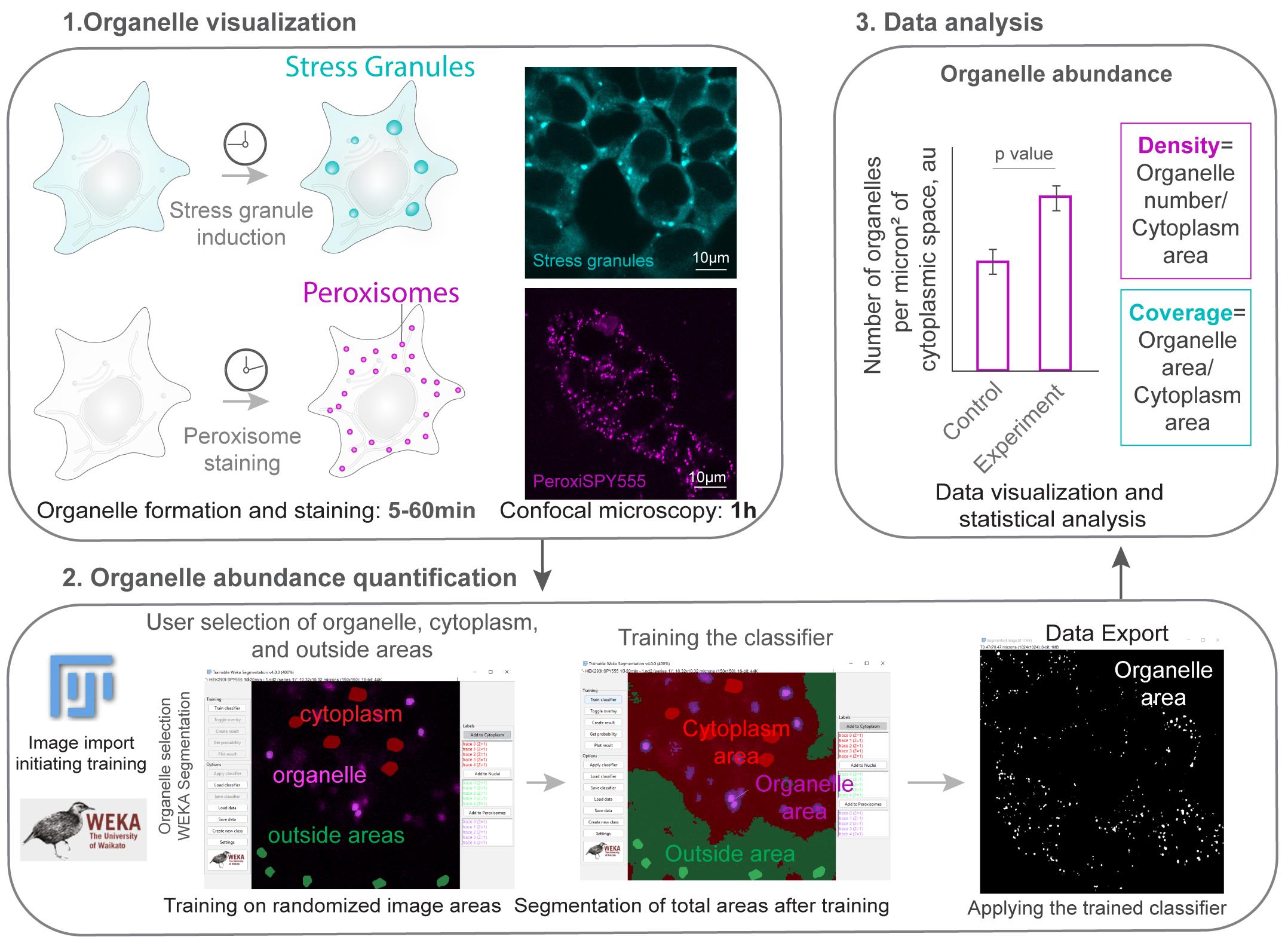
Graphical overview. Section 1 (organelle visualization) corresponds to section A in the procedure. Section 2 (organelle abundance quantification) corresponds to section B in the procedure. Section 3 (data analysis) takes place after the procedure.
Background
Quantifying organelle abundance by determining how many organelles are present in the cell and the area of the cytoplasm they cover provides a useful measure of organelle dynamics and offers insight into organelle function. For example, stress granules are membrane-less organelles that form from stalled translation pre-initiation complexes and other proteins in response to stress [1–3], with their functional roles emerging upon their assembly in the cytoplasm. Similarly, peroxisomes are membrane-enclosed organelles that are essential for lipid and oxidative metabolism [4–6]. They undergo division and increase in number when their metabolic activity is required. In both cases, quantifying organelle density in the cytoplasm correlates with organelle function in healthy cells.
Organelle abundance can be estimated from confocal imaging by visualizing resident proteins or established organelle markers [7]. An organelle marker is any fluorescently labeled molecule that localizes to an organelle. Examples include overexpressing a fluorescent protein fused to an organelle localization signal or an endogenously tagged protein. Examples of endogenously tagged proteins include the CRISPR/Cas9 genomic fusion of polyA-binding protein PABPC1 to Dendra2, which is used as a marker of stress granules [8], and ATP-binding cassette sub-family D member 3 (ABCD3) fused to GFP as a marker of peroxisomes [9]. Other examples include using a fluorescent probe that selectively targets the organelle, such as PeroxiSPY, which is used to label peroxisomes [10], or using antibody staining of organelles post-fixation [9]. The quantification requires segmentation, or defining the boundaries of compartments, which is often based on visual inspection. Manual segmentation is prone to error; for example, it is difficult to consistently outline highly variable, punctate, or overlapping patterns. To improve the reliability of quantification, thresholding methods set an intensity value independent of the user, improving consistency [11]. Machine learning approaches further reduce manual segmentation errors by providing consistent labeling based on user-defined parameters [12–14].
Here, we present a protocol for quantifying the abundance of membrane and membrane-less organelles based on a single marker using Fiji software [15,16]. This protocol combines the WEKA Segmentation [12] and watershed algorithms into a user-friendly workflow. The quantification is based on trainable organelle recognition, which limits user-defined thresholding bias and improves the consistency of image processing [14,17,18]. Recognition requires reliably outlining organelles for initial training, a task that can be done by experienced researchers. The trained classifier can then be applied to any number of images obtained with the same microscopy settings. Alternatively, a beginning researcher can train the classifier and include controls to verify whether the recognized area corresponds to an organelle area.
As a proof-of-concept, we validate that machine learning–assisted recognition of cellular compartments corresponds to an independent marker of cellular cytoplasmic and peroxisome areas using a control marker for both the organelle and the cytoplasm. In many experimental setups, adding additional markers is not feasible, and manually extracting the cytoplasmic area from a single organelle marker is biased and time-consuming. Our results demonstrate that machine learning assistance enables the consistent and reliable identification of these regions. Finally, we apply the macro to quantify the non-membrane compartment density of stress granules using a CRISPR/Cas9-tagged PABPC1 cell line [19]. The algorithm recognizes conditions in which there are no stress granule compartments and extracts areas based on a single marker.
This protocol can be modified further to estimate organelle coverage and the area of the cell occupied by the cytoplasm, or to extract abundance in 3D using stacks of 2D images obtained from tissues. This provides a useful tool for quantitative cell biology experiments.
Materials and reagents
Biological materials
Cell lines and organisms used in this study:
1. Human embryonic kidney cells HEK293T (ATCC® CRL-3216TM)
2. HEK293T PABPC1-DDR2 cell line [8]
3. Zebrafish Danio rerio
Reagents
1. PeroxiSPY555 (Spirochrome, catalog or CAS number: SC207: Peroxi_SPY555); store 1 mM stock in DMSO at -20 °C long-term; aliquots can be stored at 4 °C
2. Sodium arsenite (Thermo Fisher Scientific, catalog or CAS number: 7784-46-5)
3. Immersion liquid (Cargille, catalog or CAS number: 16482)
4. Penicillin/Streptomycin for cell culture (Pan Biotech, catalog or CAS number: P06-07050)
5. Dulbecco’s modified Eagle’s medium (DMEM) cell culture media with 10% fetal bovine serum (FBS) (Pan Biotech, catalog or CAS number: P30-3031, P04-03590)
6. DMSO (Invitrogen, catalog number: D12345)
Solutions
1. 200 μM sodium arsenite in media (see Recipes)
2. 1 μM PeroxiSPY in DMEM (see Recipes)
Recipes
1. 200 μM sodium arsenite in media
To dissolve in tissue culture medium, add 2 μL of the 100 mM stock in water to 1 mL of medium. Mix by vortex mixing or pipetting before adding to the cells.
2. 1 μM PeroxiSPY in DMEM
To dissolve PeroxiSPY in media, add 1 μL of the 1 mM stock to an Eppendorf tube, then add 1 mL of DMEM. Mix by vortex mixing or pipetting before adding to the cells.
Laboratory supplies
1. 4-chamber glass bottom plates (CellVis, catalog number: D35C4200N), cover glass (0.13–0.16 mm), used for confocal imaging
2. Tissue culture 10 cm plates (Sigma) used for cell culture
Note: Plastic plate thickness will not allow confocal imaging at 60×; however, larger organelles can be imaged through plastic plates at a lower magnification, e.g., 20×, e.g., for nuclei segmentation.
Equipment
1. Confocal microscope (Nikon, model: A1r), equipped with a CFI Plan Apo Lambda 60× oil NA 1.42 objective
2. Spinning disk microscope (Nikon, model: W1), equipped with a CFI Plan Apochromat Lambda S 60XC Sil objective
3. CO2 chamber and temperature control unit (OKO Lab, model: CO2-O2 Unit-BL)
4. CO2 incubator for cell culture (Thermo Fisher Scientific, model: Steri-Cycle CO2 incubator: 370)
5. Eppendorf tubes
Software and datasets
1. Example dataset, 01.12.2025, free: Supplementary Dataset S1
2. Fiji software (or ImageJ), Java 21.0.7 (64-bit), 01.12.2025, free [15,16]
3. NIS Nikon software, 4.1, paid (microscope software)
4. Macro (organelle abundance algorithm), resource, 1.0, 01.12.2025, free: Supplementary Code S1
Procedure
A. Image acquisition and wet-lab component of the protocol
Cell culture preparation for live-cell imaging (timing: 24 h)
To begin the procedure (Figure 1), we obtained microscopical images of organelles of interest. To prepare for confocal imaging, we used standard cell culture protocols.
HEK293T cells were maintained in high-glucose DMEM media supplemented with 10% fetal bovine serum (FBS), 1% penicillin/streptomycin, at 37 °C/5% CO2. The media was replaced every 2nd day; the cells were seeded at a density of 50,000 cells per a well of a 4-well imaging plate. Cells were visualized at a 50–70% confluency, cells were split before they reached 90% confluency.
Caution: If your microscope detects the signal from phenol red in the media, use phenol red-free alternatives, e.g., P04-01158 (Pan Biotech).
1. One day before image acquisition, split the cells into a glass-bottom imaging plate to achieve 50%–60% confluency the next day. We split HEK293T for peroxisome staining and HEK293T PABPC1-DDR2 for stress granule imaging at a density of 50,000 cells per well of the microscopy plate.
2. Live-cell image acquisition (timing: 1 h): Imaging organelles requires high spatial resolution. For this protocol, we used the Nikon A1r confocal microscope equipped with gallium arsenide phosphide cathodes (GaAsP) photomultiplier modules, a CO2 chamber, and a temperature control unit. Imaging was done using a bi-directional Galvano-scanning mode using CFI Plan Apo Lambda 60× oil NA 1.42 objective, using a 561 nm laser (Coherent, 50 mW) for PeroxiSPY555 and a 488 nm laser (Coherent, 50 mW) for DDR2.
a. Turn on the microscope, the required lasers, and the CO2/temperature units. Ensure that the CO2 and temperature (37 °C) are stabilized for at least 15 min before imaging.
b. Initiate the software and adjust the software parameters for acquisition. We used 0.5%–2% laser power and HV (gain) of 100, and acquired 1024 × 1024 px, zoom 3–4× images.
Note: To ensure maximum resolution, we recommend following Nyquist sampling [21]: adjust the pixel size to be 2.3 times smaller than the smallest compartment that you are imaging. Increasing HV (gain) will increase the brightness but will also increase the noise. To ensure that data is usable, the same imaging parameters should be applied to all images within one experiment. Any confocal microscope can be used for this protocol.
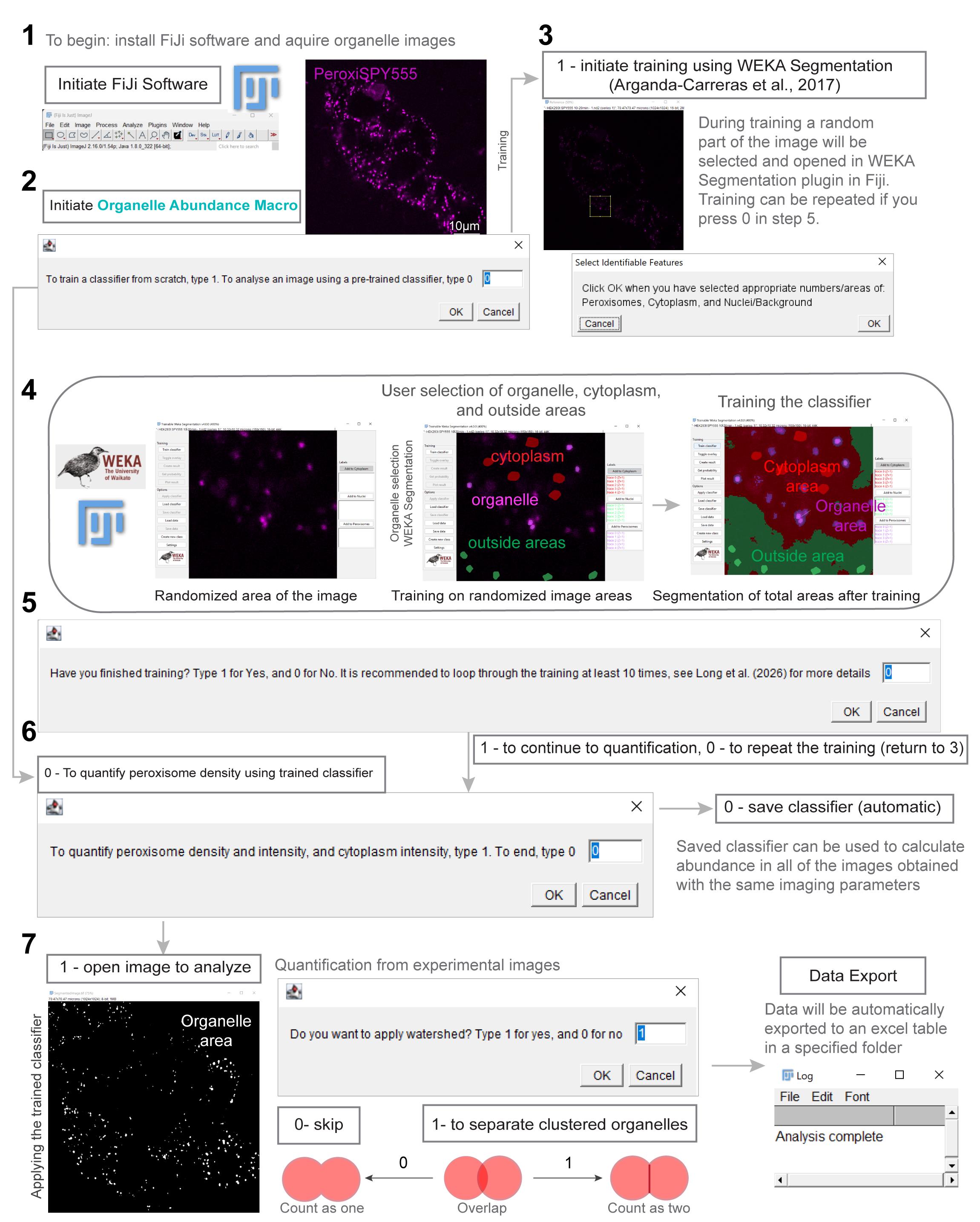
Figure 1. Organelle abundance quantification workflow (Code S1). Figure number 1 corresponds to section A; number 2 corresponds to steps B1a–1d; number 3 corresponds to step B1e, number 4 corresponds to steps B1f–1i; number 5 corresponds to step B1j; number 6 corresponds to steps B2a–2c; and number 7 corresponds to step B2d.
3. Staining and acquiring of the organelle images.
a. Stress granule imaging requires inducing the formation of stress granules, as previously described [19]. Pipette a 100 mM sodium arsenite solution (see Recipes) as a 1/500 part of your total media volume in an empty Eppendorf tube, e.g., for 0.5 mL of media, pipette 1 μL of arsenite. Collect the media from the cells and mix with sodium arsenite by vortex mixing or pipetting. After mixing, add the mix to the plate and incubate for 1 h in the cell culture incubator. For peroxisome imaging, stain cells with PeroxiSPY for 10 m as previously described [10,21]. To incubate the cells with 1 μM of PeroxiSPY555 (see Recipes), pipette 1 mM PeroxiSPY aliquot as a 1/1,000 part of your total media volume in an empty Eppendorf tube, e.g., for 0.5 mL of media, pipette 0.5 μL of PeroxiSPY. Collect the media from the chosen microscope plate and mix with PeroxiSPY by vortex mixing or pipetting. After mixing, add the mix to the plate and incubate for 5–10 min.
Caution: Do not leave the cells without media for more than 20 s to avoid osmotic stress. To achieve uniform staining and organelle formation, all the media should be mixed with the molecules.
b. Add immersion liquid to the objective (we use a 60× oil objective) and position the plate. Adjust focus until the cells are visible and in focus. Randomly choose an imaging area and adjust the acquisition parameters (e.g., HV-100, laser power = 1%, zoom 3, 1024 × 1024 px, scan speed 1/2–1/4).
c. Acquire and save all images with accessible labels (we use .nd2 Nikon NIS Software), including cell line, staining, genetic modification, treatment, and time, if applicable.
Pause point: Images can be stored and processed when needed.
Notes:
1. Stress granule formation: To visualize stress granules, replace the media in the glass-bottom plate for live-cell imaging with 200 μM sodium arsenite dissolved in the cell culture media and incubate for 1 h in the cell culture incubator at 37 °C/5% CO2 [19]. To prepare 200 μM sodium arsenite, dissolve 2 μL of 100 mM sodium arsenite stock in water in 1 mL of media, use vortex mixing or pipetting.
2. Peroxisome staining: Peroxisomes were stained with PeroxiSPY [10], as described in [22]. To visualize peroxisomes, replace the media in the glass-bottom plate for live-cell imaging with 1 μM PeroxiSPY dissolved in the cell culture media and incubate for 5–10 m in the cell culture incubator at 37 °C/5% CO2.
B. Image analysis: quantification of organelle density
1. Training the classifier for organelle abundance quantification: A classifier is an algorithm or model used to classify data [23]. In the Fiji software, this is stored as a “.model” file and is used by the Trainable Weka Segmentation tool to classify sections of an image into organelles, cytoplasm, and the area outside of the cytoplasm.
a. Open the macro file in Fiji (Supplementary code S1), either by dragging the file onto the Fiji window or by clicking File > Open on the Fiji window.
b. Once the macro editor window appears, open the window full-screen and click Run in the lower-left corner.
c. Follow the prompt on the pop-up window. Type “1” in the dialog box to train a classifier from scratch, or type “0” to use a pre-trained classifier. If you type “0”, skip to step B2a.
Note: To open .nd2 images, you will need to install the .nd2 reader in Fiji (https://imagej.net/ij/plugins/nd2-reader.html).
d. Using the pop-up window, select the folder containing your training image, ensuring this folder contains only the training image, and a folder in which to store the trained classifier and training data. Ensure that this second folder is empty.
e. Wait for the macro to run until a small window titled “Select Identifiable Features” appears. Additionally, two other important windows will appear, titled “Trainable Weka Segmentation” [12] and “Reference.”
f. Using the “Trainable Weka Segmentation” window and the “Reference” window for clarity, draw around up to five visible organelles, depending on how many are visible. Click the Add to Organelles button on the right side of the window before drawing around each subsequent one.
Note: Peroxisomes are ~0.5 μm round compartments in the cytoplasm that co-localize with peroxisome marker GFP-SKL in healthy cells (Figure 2A). When drawing in Weka segmentation, only select the area that corresponds to peroxisomes. Avoid overdrawing.
g. After selecting up to five visible organelles, select five sections of cytoplasm, each at least the size of the organelles selected in step B1f. Click the Add to Cytoplasm button on the right side of the window before drawing around each subsequent area.
h. Finally, select five sections outside of the cytoplasm, each at least the size of the organelles selected in step B1f. Click the Add to Nuclei button on the right side of the window before drawing around each subsequent area.
i. Click the OK button in the “Select Identifiable Features” window and wait until training has been completed. To identify if the training has been completed, wait until the image displayed in the “Trainable Weka Segmentation” window changes to highlight the organelles (purple), cytoplasm (red), and nuclei/background (green).
j. A new window will appear, asking to continue or finish training. Type “1” into the dialog box to finish training, and type “0” to continue training. We recommend repeating the training steps (steps B1f–B1i) nine additional times, totaling 10 training loops. This number is based on data from Figure 2B, which suggests that after 10 training loops, the change in identified area was minimal.
2. Using the Macro to analyze an image: The macro will use the trained classifier (B1a–B1j) and a watershed function to automatically determine the area and intensity of the visible organelles and cytoplasm and the abundance of the visible organelles.
a. A pop-up window will appear asking whether you wish to analyze a new image using the previously trained classifier. Type “1” to continue with organelle analysis or “0” to stop the macro. Stopping the macro is recommended if you wish to analyze more than one image. Typing “0” will result in the text “Training complete” being displayed.
b. In the next pop-up window titled “Select your Files,” select the folder containing the image you wish to analyze. Ensure this folder contains only one image. Then, select a folder to save the results, ensuring this folder is empty.
c. This step is only applicable if you are using a pre-trained classifier (if steps B1d–B1j were skipped). The same pop-up window described in step B1d will appear with an additional field. Select the folder that contains the pre-trained classifier. This folder should contain two files in the form of a classifier file (ending in .model) and a data file.
d. Wait for the analysis section of the macro to run until a pop-up window asks whether you want to apply Fiji’s watershed tool to the organelles. This will attempt to separate organelles that are too close, ensuring they are counted separately. This is useful in samples with high organelle density; higher density of organelles increases the likelihood of organelles overlapping and thus causing the macro to count fewer than are present in the image. Type “1” for yes and “0” for no.
e. Wait until the text “Analysis complete” displays in the “log” window.
Result interpretation
The expected output from this protocol is an Excel table with the list of detected organelles (Supplementary Table 1), their areas, and corresponding average intensity per area, with a calculated density of organelles in the cytoplasm in the form of the number of organelles per square micron (abundance). Results can be plotted as a distribution of organelle areas (Figure 2A) or densities (Figure 3A). Coverage of the area can be extracted by dividing the sum of organelle areas by the sum of organelle and cytoplasmic areas.
Image quality determines whether the data are usable and quantifiable. Image quality depends on the sample preparation and correct microscopy settings. For each organelle, we recommend consulting with the literature on the expected size and number of the organelles in the cell line of choice. When imaging organelles for the first time, ensure that you have a verified organelle marker as a control (Figure 2A). To ensure maximum resolution, adjust the microscope settings to ensure that the pixel size is at least 2.3 times smaller than the smallest compartment that you are imaging. This can be done by increasing the image size or physical zoom. Avoid saturation of the organelle areas and ensure that the background noise is minimized by reducing the gain. The protocol estimates cytoplasmic areas based on the residual fluorescence; it is recommended to confirm whether the cytoplasmic area corresponds to the actual cytoplasmic area using secondary markers (Figure 2A).
It is recommended to perform at least three biological replicates to obtain the data. The same classifier can be used to quantify the areas in all the images obtained with the same imaging parameters. Additionally, it is recommended to quantify organelle areas in at least 100 cells per condition. If the data follows a normal distribution, determined by the Shapiro–Wilk test, P values can be calculated using a two-tailed Student’s t-test for two samples or a one-way ANOVA for multiple samples. The equality of variances can be verified by the Brown–Forsythe or F test. Mann–Whitney (two groups) or Kruskal–Wallis (multiple groups) tests can be used for samples that do not follow a normal distribution. Sample sizes can be determined using power analysis. Results obtained from images with different microscopy parameters cannot be reliably compared (Figure 2C).
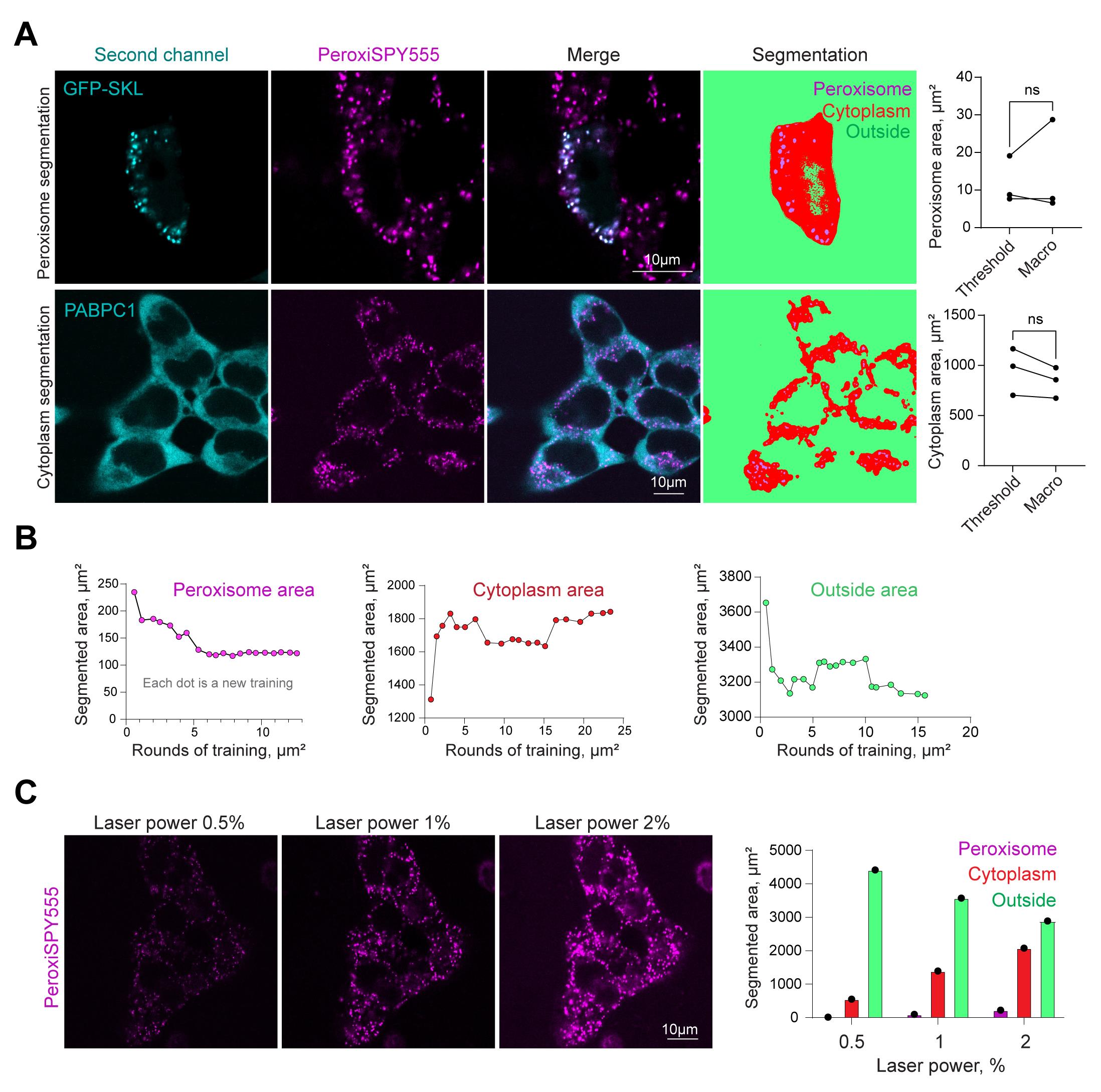
Figure 2. Protocol validation. (A) Confocal microscopy of peroxisomes in HEK293T cells (upper row) expressing peroxisome marker GFP-SKL, stained with PeroxiSPY (1 μM for 10 m) or (bottom row) expressing CRISPR/Cas9 PABPC1-DDR2 and stained with PeroxiSPY(1 μM for 10 m). Segmentation panels (fourth column) show areas recognized by the classifier. Quantification shows the area size detected with the manual threshold method and the area segmented by the classifier. N = 3, mean ± SEM; ns: non-significant. (B) Determination of segmented areas and the number of sequential training loops required for appropriate classifier training. Each dot represents an additional training area, including the data from the previous training. (C) Confocal microscopy of peroxisomes in HEK293T cells stained with PeroxiSPY (1 μM for 10 min) imaged with 0.5%, 1%, or 2% laser power. Quantification shows the area size detected with the classifier trained on laser power 1% image.
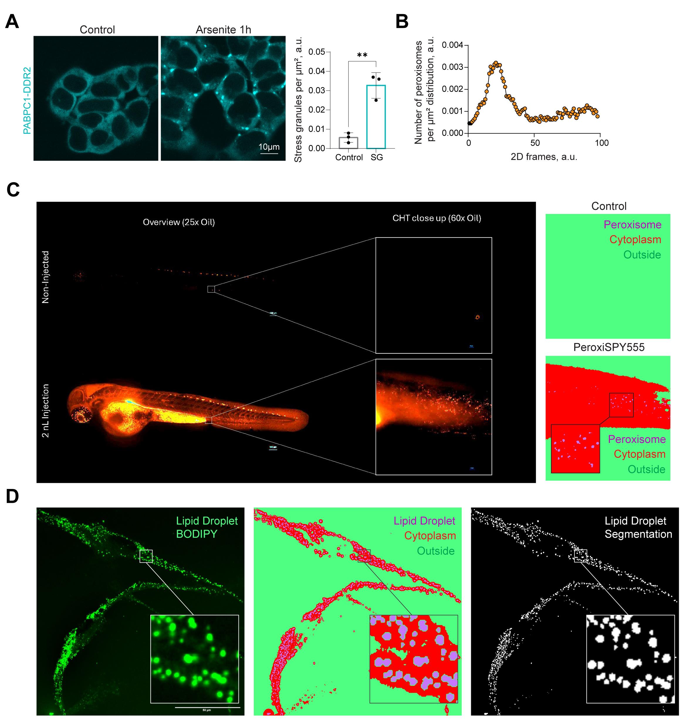
Figure 3. Protocol application. (A) Confocal microscopy of stress granules in HEK293T PABPC1-DDR2 cells in control and 200 μM arsenite (60 min) conditions. Quantification shows the cytoplasmic density of stress granules. N = 3, mean ± SEM. **p < 0.01. (B–C) Confocal images of zebrafish embryos at 3 days post-fertilization injected with 2 nL of PeroxySpy555 at 1 mM in the blood circulation by the duct of Cuvier. Images were acquired 2 h after injection, using a W1 Nikon Spinning disk microscope. Images were segmented using the macro, and peroxisomal areas were detected and plotted on the histogram (B). (D) Macro-based segmentation of lipid droplets in human iPSC-derived microglia. Representative fluorescence image of human iPSC-derived microglia at day 21 of differentiation (D21) stained with BODIPY 493/503 to label lipid droplets. Corresponding WEKA segmentation and binary segmentation mask generated using the custom macro; white indicates segmented lipid droplets, and black denotes cytoplasm/background. Scale bars, 50 μm.
Validation of protocol
We confirmed that machine learning–assisted area segmentation corresponds to the physical cytoplasmic and organelle space using secondary markers (Figure 2A). Peroxisomal area quantified using the organelle abundance macro is the same as a manually thresholded area defined by a GFP-SKL peroxisomal marker in the same cells (Figure 2A).
The segmentation relies on intensity; therefore, it is recommended to train the classifier for each set of imaging parameters, such as laser power or exposure. It takes only 5–10 training cycles, using the random area of the same image (Figure 1, Figure 2B), to reliably train the classifier. We showed that increased laser power corresponds to a gradual increase in areas recognized by the classifier (Figure 2C), thereby requiring classifier training for each independent dataset.
The classifier, once trained, can be applied to a necessary number of repeats of images obtained with the same microscope settings; at least 3 biological replicates were done for the experiments presented here. We applied a stress granule–trained classifier to identify stress granule density in control and stress conditions (Figure 3A). The macro allowed the extraction of the absence of stress granules from all control images.
This tool extracts organelle abundance data from 2D images. 3D space abundance can be extracted from a Z-stack of 2D images. Here, we estimated peroxisome density in zebrafish D. rerio injected with PeroxiSPY peroxisome probes (Figure 3B). Additionally, this protocol can be applied to other cellular organelles in different cell types, resulting in their reliable segmentation (Figure 3D, lipid droplets in neuronal cells).
As limitations, the protocol relies on the user to define the organelle to be classified; after that, the procedure is not user-biased. It is, therefore, recommended that the classifier be trained by either an experienced researcher or a beginning researcher who compares their classifier data to a secondary marker to ensure that the area corresponds to the organelle area of interest (see Figure 2A). Caution should be applied when estimating the absolute coverage of organelles. As we show in Figure 2C, it depends on imaging parameters. Quantification of relative coverage, including negative and positive controls, is recommended, e.g., organelle abundance between conditions imaged with the same microscopy parameters (e.g., Figure 3A).
To ensure independent validation, we provide a dataset to train and apply the classifier (Supplementary dataset S1), which includes two images for training and detection; additionally, Supplementary table S1 includes expected results.
General notes and troubleshooting
General notes
1. The classifiers used in this protocol are trained on data using the macro (code S1) and can be used to estimate organelle abundance. Users can also follow the training algorithm to train their own classifier to be applied in different conditions or for a different cellular compartment.
2. The protocol has been tested in several microscope settings (e.g., laser power changes), using several organelle markers. Its applicability to a different organelle needs to be confirmed with a secondary marker, as we have done in Figure 2.
3. It is recommended to train the classifier for 5–10 loops on each dataset (using a representative image) with new microscopy parameters.
4. Zebrafish husbandry and ethics: All zebrafish were raised at the University of York in UK Home Office-approved aquaria and maintained following a standard protocol [20]. Tanks were maintained at 28 °C with a continuous re-circulating water supply and a daily light/dark cycle of 14/10 h. The nacre WT background strain was used to perform injections.
Troubleshooting
Problem 1: Unable to detect organelle areas.
Possible cause: Image quality is low.
Solution: Optimize the imaging acquisition parameters. For example, HV (gain) will increase brightness but will also increase noise. Increase laser power and decrease gain to improve the signal-to-noise ratio.
Possible cause: Photobleaching.
Solution: Some fluorescent molecules are photostable (e.g., PeroxiSPY), while others can bleach with laser exposure (e.g., DDR2). Reduce light exposure when handling samples by wrapping the plate in aluminum foil or working in the dark room. When imaging, do not image the same area repeatedly. Find the area on a low laser power setting and then switch to the higher laser power setting before acquiring the final image. Use mounting media with antifade protection if using fixed samples.
Problem 2: Organelle areas are too big.
Possible cause: User-defined areas are not specific to the organelle during the selection process.
Solution: Select areas strictly within the organelle.
Possible cause: Oversaturation.
Solution: When setting microscopy parameters, avoid saturation by reducing the gain and laser power until only a few or no pixels remain saturated.
Problem 3: Organelle cluster prevents the quantification of the numbers.
Possible cause: Watershed is not applied during the procedure (step B2d, type 1 to apply).
Solution: Apply the watershed that separates clusters into separate compartments.
Problem 4: Not enough organelles are visible while training.
Possible cause: The randomly selected training area is too small.
Solution: Navigate to lines 4 and 5 in the macro while it is open in Fiji and not running. Edit lines 4 and 5 in the macro so that “w” and “h” variables are larger. For example, lines 4 and 5 could be replaced with:
Line 4: “w = 250;”
Line 5: “h = 250;”
Supplementary information
The following supporting information can be downloaded here:
1. Dataset S1. Example images to train and quantify the density of peroxisomes.
2. Code S1. Macro to quantify organelle abundance.
3. Table S1. Example output results table.
4. Video S1. Video explanation of the workflow.
Acknowledgments
Conceptualization, A.J.L. and T.A.; Investigation, A.J.L., D.C., N.H., L.R., M.S., N.F.C., and T.A.; Writing—Original Draft, A.J.L. and T.A.; Writing—Review & Editing, A.J.L., D.C., N.F.C., N.H., M.S., L.R., S.K., and T.A.; Funding acquisition, S.K. and T.A.; Supervision, N.H., M.S., S.K., and T.A.
We thank the School of Biological Sciences Imaging and Microscopy Centre (IMC) for providing access to essential equipment. T.A. was funded by the HFSP Long-term Fellowship (LT000559/2021-L), the University of Southampton, the Wessex Medical Research Innovation Grant, and the European Leukodystrophy Association (ELA International: grant number 2024-017C1A to S.K. and T.A.).
The protocol was derived from peroxisome density calculations in [9] and [10].
We thank David S. Chatelet for providing insights into the Fiji macro language. We thank Prof. Dr. V.M. Heine (Amsterdam UMC and Vrije Universiteit Amsterdam) for providing access to microscopy images of iPSC-derived microglia stained for lipid droplets, which were used for validation.
Public forums utilized in the organelle abundance macro: Reddit.com, Image.sc, imagej.273.s1.nabble.com, and ImageJ.net.
Competing interests
The authors declare no conflicts of interest.
References
- Ivanov, P., Kedersha, N. and Anderson, P. (2018). Stress Granules and Processing Bodies in Translational Control. Cold Spring Harbor Perspect Biol. 11(5): a032813. https://doi.org/10.1101/cshperspect.a032813
- Protter, D. S. and Parker, R. (2016). Principles and Properties of Stress Granules. Trends Cell Biol. 26(9): 668–679. https://doi.org/10.1016/j.tcb.2016.05.004
- Riggs, C. L., Kedersha, N., Ivanov, P. and Anderson, P. (2020). Mammalian stress granules and P bodies at a glance. J Cell Sci. 133(16): e242487. https://doi.org/10.1242/jcs.242487
- Kumar, R., Islinger, M., Worthy, H., Carmichael, R. and Schrader, M. (2024). The peroxisome: an update on mysteries 3.0. Histochem Cell Biol. 161(2): 99–132. https://doi.org/10.1007/s00418-023-02259-5
- Wanders, R. J. and Waterham, H. R. (2006). Biochemistry of Mammalian Peroxisomes Revisited. Annu Rev Biochem. 75(1): 295–332. https://doi.org/10.1146/annurev.biochem.74.082803.13332
- Wanders, R. J. A., Waterham, H. R. and Ferdinandusse, S. (2018). Peroxisomes and Their Central Role in Metabolic Interaction Networks in Humans. Subcellular Biochemistry. 89: 345–365. https://doi.org/10.1007/978-981-13-2233-4_15
- Metz, J., Castro, I. and Schrader, M. (2017). Peroxisome Motility Measurement and Quantification Assay. Bio Protoc. 7(17): e2536. https://doi.org/10.21769/bioprotoc.2536
- Amen, T. and Kaganovich, D. (2021). Stress granules inhibit fatty acid oxidation by modulating mitochondrial permeability. Cell Rep. 35(11): 109237. https://doi.org/10.1016/j.celrep.2021.109237
- Borisyuk, A., Howman, C., Pattabiraman, S., Kaganovich, D. and Amen, T. (2025). Protein Kinase C promotes peroxisome biogenesis and peroxisome–endoplasmic reticulum interaction. J Cell Biol. 224(9): e202505040. https://doi.org/10.1083/jcb.202505040
- Korotkova, D., Borisyuk, A., Guihur, A., Bardyn, M., Kuttler, F., Reymond, L., Schuhmacher, M. and Amen, T. (2024). Fluorescent fatty acid conjugates for live cell imaging of peroxisomes. Nat Commun. 15(1): 4314. https://doi.org/10.1038/s41467-024-48679-2
- Russell, R. A., Adams, N. M., Stephens, D. A., Batty, E., Jensen, K. and Freemont, P. S. (2009). Segmentation of Fluorescence Microscopy Images for Quantitative Analysis of Cell Nuclear Architecture. Biophys J. 96(8): 3379–3389. https://doi.org/10.1016/j.bpj.2008.12.3956
- Arganda-Carreras, I., Kaynig, V., Rueden, C., Eliceiri, K. W., Schindelin, J., Cardona, A. and Sebastian Seung, H. (2017). Trainable Weka Segmentation: a machine learning tool for microscopy pixel classification. Bioinformatics. 33(15): 2424–2426. https://doi.org/10.1093/bioinformatics/btx180
- Lam, V. K., Byers, J. M., Robitaille, M. C., Kaler, L., Christodoulides, J. A. and Raphael, M. P. (2025). A self-supervised learning approach for high throughput and high content cell segmentation. Commun Biol. 8(1): e1038/s42003–025–08190–w. https://doi.org/10.1038/s42003-025-08190-w
- Lefebvre, A. E. Y. T., Sturm, G., Lin, T. Y., Stoops, E., López, M. P., Kaufmann-Malaga, B. and Hake, K. (2025). Nellie: automated organelle segmentation, tracking and hierarchical feature extraction in 2D/3D live-cell microscopy. Nat Methods. 22(4): 751–763. https://doi.org/10.1038/s41592-025-02612-7
- Schindelin, J., Arganda-Carreras, I., Frise, E., Kaynig, V., Longair, M., Pietzsch, T., Preibisch, S., Rueden, C., Saalfeld, S., Schmid, B., et al. (2012). Fiji: an open-source platform for biological-image analysis. Nat Methods. 9(7): 676–682. https://doi.org/10.1038/nmeth.2019
- Schneider, C. A., Rasband, W. S. and Eliceiri, K. W. (2012). NIH Image to ImageJ: 25 years of image analysis. Nat Methods. 9(7): 671–675. https://doi.org/10.1038/nmeth.2089
- Isensee, F., Jaeger, P. F., Kohl, S. A. A., Petersen, J. and Maier-Hein, K. H. (2020). nnU-Net: a self-configuring method for deep learning-based biomedical image segmentation. Nat Methods. 18(2): 203–211. https://doi.org/10.1038/s41592-020-01008-z
- Newby, J. M., Schaefer, A. M., Lee, P. T., Forest, M. G. and Lai, S. K. (2018). Convolutional neural networks automate detection for tracking of submicron-scale particles in 2D and 3D. Proc Natl Acad Sci USA. 115(36): 9026–9031. https://doi.org/10.1073/pnas.1804420115
- Amen, T. and Kaganovich, D. (2020). Quantitative photoconversion analysis of internal molecular dynamics in stress granules and other membraneless organelles in live cells. STAR Protoc. 1(3): 100217. https://doi.org/10.1016/j.xpro.2020.100217
- Cunliffe, V. (2003.) Zebrafish: A Practical Approach. Edited by C. NÜSSLEIN-VOLHARD and R. DAHM. Genetics Research. 82: 79. https://doi.org/10.1017/S0016672303216384
- Shannon, C. (1949). Communication in the Presence of Noise. Proc IRE. 37(1): 10–21. https://doi.org/10.1109/jrproc.1949.232969
- Howman, C., Cohen, T., Shlomy, M. Y., van Aerle, M. S., Carmichael, R. E., Schuhmacher, M., Reymond, L., Zalckvar, E., Kaganovich, D., Amen, T., et al. (2025). Peroxisome Staining in Mammalian Cells Using Peroxisome-Specific Probes. J Visualized Exp. e3791/69405. https://doi.org/10.3791/69405
- Bi, Q., Goodman, K. E., Kaminsky, J. and Lessler, J. (2019). What is Machine Learning? A Primer for the Epidemiologist. Am J Epidemiol. 188: 2222–2239. https://doi.org/10.1093/aje/kwz189
Article Information
Publication history
Received: Dec 7, 2025
Accepted: Jan 28, 2026
Available online: Feb 12, 2026
Published: Mar 5, 2026
Copyright
© 2026 The Author(s); This is an open access article under the CC BY-NC license (https://creativecommons.org/licenses/by-nc/4.0/).
How to cite
Readers should cite both the Bio-protocol article and the original research article where this protocol was used:
- Long, A. J., Candeias, D., Coveña, N. F., Reymond, L., Schuhmacher, M., Kemp, S., Hamilton, N. and Amen, T. (2026). Machine Learning-Assisted Quantification of Organelle Abundance. Bio-protocol 16(5): e5626. DOI: 10.21769/BioProtoc.5626.
- Borisyuk, A., Howman, C., Pattabiraman, S., Kaganovich, D. and Amen, T. (2025). Protein Kinase C promotes peroxisome biogenesis and peroxisome–endoplasmic reticulum interaction. J Cell Biol. 224(9): e202505040. https://doi.org/10.1083/jcb.202505040
Do you have any questions about this protocol?
Post your question to gather feedback from the community. We will also invite the authors of this article to respond.