- Protocols

- Articles and Issues
- For Authors
- About
- Become a Reviewer

CAPS-Based SNP Genotyping for Nitrogen-Response Phenotypes in Maize Hybrids
Published: Vol 15, Iss 24, Dec 20, 2025 DOI: 10.21769/BioProtoc.5551 Views: 589
Reviewed by: Samik BhattacharyaAthanas GuzhaAnonymous reviewer(s)
Advertisement


Protocol Collections
Comprehensive collections of detailed, peer-reviewed protocols focusing on specific topics


Abstract
A simple and effective method to identify genetic markers of yield response to nitrogen (N) fertilizer among maize hybrids is urgently needed. In this article, we describe a detailed methodology to identify genetic markers and develop associated assays for the prediction of yield N-response in maize. We first outline an in silico workflow to identify high-priority single-nucleotide polymorphism (SNP) markers from genome-wide association studies (GWAS). We then describe a detailed methodology to develop cleaved amplified polymorphic sequences (CAPS) and derived CAPS (dCAPS)-based assays to quickly and effectively test genetic marker subsets. This protocol is expected to provide a robust approach to determine N-response type among maize germplasm, including elite commercial varieties, allowing more appropriate on-farm N application rates, minimizing N fertilizer waste.
Key features
• Leverages GWAS datasets to efficiently identify genetic markers.
• Employs basic molecular biology techniques.
• Can be adapted to any maize germplasm.
Keywords: SNPGraphical overview
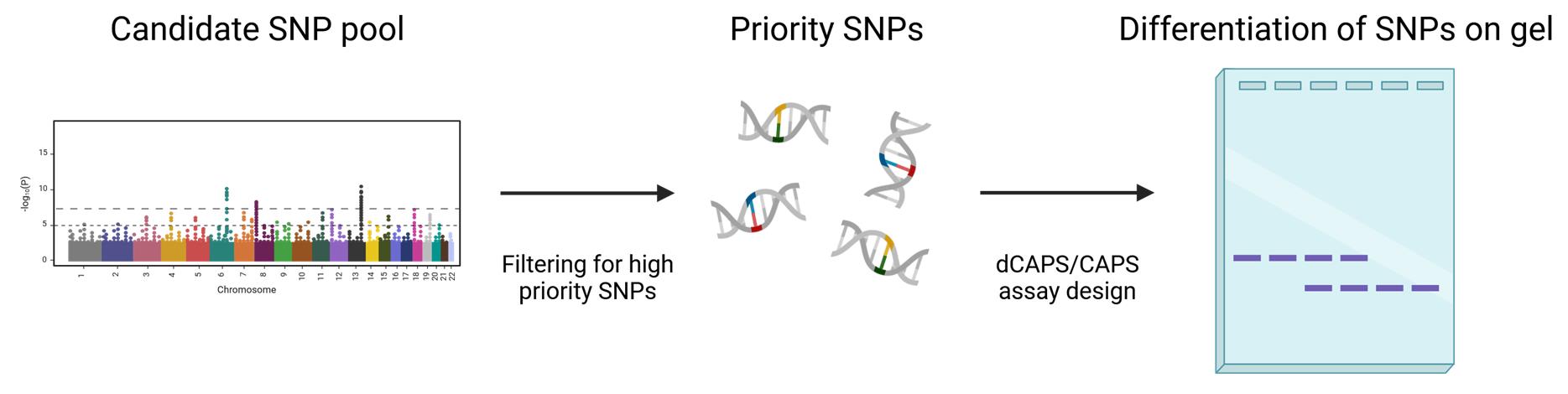
Visual description of the pipeline describing how to prioritize and visualize single-nucleotide polymorphisms (SNPs)
Background
Maize production systems are heavily reliant on the provision of N fertilizer to maximize growth and yield. However, the yield gain from N applications can vary widely depending on the underlying genetics. Certain hybrids, known as Type 3 hybrids, continue to increase yield even at very high N application rates, while others, known as Type 1 hybrids, hit a yield plateau at relatively low N application rates, meaning additional N is largely ineffective at increasing yield [1]. Knowledge of N-response type is highly valuable to a farmer, as it allows them to tailor their N application rates to match what the maize can utilize, thus minimizing financial and environmental costs. However, determination of N-response type currently requires time- and labor-intensive field tests spanning multiple years. A genetic marker–based approach to determine yield N-response of maize germplasm would be much faster and easily accessible for breeders and farmers.
Here, we describe a simple and effective protocol to identify candidate single-nucleotide polymorphism (SNP) markers associated with yield N-response type and to develop cleaved amplified polymorphic sequences (CAPS) assays to genotype these markers [2]. The following protocol begins with in silico filtering of SNP marker data that may have come from, for example, genome-wide association studies (GWAS). The filtering prioritizes candidate SNPs, essential to avoid repetitive or duplicated regions, which are less accessible to marker assays. A suitable CAPS assay is then developed to genotype candidate SNPs. The CAPS method relies on restriction enzyme cleavage that differentiates (i.e., cutting or not cutting) depending on the nucleotide at a particular SNP. As an alternative approach, when the SNPs do not present a suitable site for restriction digestion, the derived CAPS (dCAPS) approach can be employed [3]. In either case, a region encompassing the SNP is amplified and digested using a restriction enzyme before being separated by gel electrophoresis as a read-out of the SNP identity.
Materials and reagents
Biological materials
1. B73, Zea mays L. subsp. mays (USDA National Plant Germplasm System, PI 550473 2024ncai01 SD)
2. LH195, Zea mays L. subsp. mays (USDA National Plant Germplasm System, PI 537097 13ncai01 SD)
3. PHN82, Zea mays L. subsp. mays (USDA National Plant Germplasm System, PI 601783 2022ncai01 SD)
4. PHB47, Zea mays L. subsp. mays (USDA National Plant Germplasm System, PI 601009 11ncai01 SD)
5. Mo17, Zea mays L. subsp. mays (USDA National Plant Germplasm System, PI 558532 08ncai02 SD)
6. PHK76, Zea mays L. subsp. mays (USDA National Plant Germplasm System, PI 601496 07ncai01 SD)
7. Additional maize germplasms of interest
Reagents
1. DNeasy Plant Mini kit (Qiagen, catalog number: 69104)
2. SYBR Safe DNA gel stain (Invitrogen, catalog number: S33102); store at room temperature or 4 °C away from light
3. Agarose LE (molecular biology grade) (GoldBio, catalog number: A201100)
4. Tris base (GoldBio, catalog number: T-400-500)
5. Disodium EDTA (Invitrogen, catalog number: 15576-028)
6. Acetic acid, glacial (Supelco, catalog number: AX0073-9)
7. Restriction enzymes, as necessary (New England Biolabs Inc., various catalog numbers); store at -20 °C
8. Restriction enzyme buffers, as necessary (New England Biolabs Inc., various catalog numbers); store at -20 °C
9. Nuclease-free water (Promega, catalog number: MC1191)
10. GoTaq Green Master Mix (Promega, catalog number: M7122); store at -20 °C
11. GoTaq Colorless Master Mix (Promega, catalog number: M7132); store at -20 °C
12. Milli-Q water
Solutions
1. 5× TAE buffer (see Recipes)
2. 0.5× TAE (see Recipes)
3. SYBR Safe incubation solution (see Recipes)
Recipes
1. 5× TAE buffer
| Reagent | Final concentration | Quantity or volume |
|---|---|---|
| Milli-Q water | n/a | ~800 mL |
| Tris base | 200 mM | 24.22 g |
| Disodium EDTA | 5.5 mM | 1.86 g |
| Glacial acetic acid | 0.6% v/v | 6.05 mL |
| Milli-Q water | n/a | Up to 1 L |
| Total | n/a | 1 L |
Adjust pH to 8.3 using KOH or NaOH. Store at room temperature. Stable for up to one month.
2. 0.5× TAE
| Reagent | Final concentration | Quantity or volume |
|---|---|---|
| 5× TAE buffer | 10% v/v | 1 L |
| Milli-Q water | n/a | 9 L |
| Total | n/a | 10 L |
Store at room temperature. Stable for up to one month.
3. SYBR Safe incubation solution
| Reagent | Final concentration | Quantity or volume |
|---|---|---|
| SYBR Safe | 0.1% v/v | 10 μL |
| Milli-Q water | n/a | 100 mL |
Store away from light at room temperature. Prepare no more than 2 h ahead of use.
Laboratory supplies
1. Olympus 0.2 mL 8-strip PCR tubes, V-seal caps (Genesee Scientific, catalog number: 27-426)
2. 1.5 mL microcentrifuge tubes (Dot Scientific, catalog number: 509-FTG)
3. Universal fit tips, 1,000 μL (VWR, catalog number: 89425-636)
4. Universal fit tips, 200 μL (VWR, catalog number: 89140-896)
5. Universal fit tips, 10 μL (VWR, catalog number: 89425-654)
Equipment
1. Horizontal mini gel electrophoresis system (Fisherbrand, catalog number: 14-955-170)
2. T100 thermal cycler (Bio-Rad, catalog number: 1861096)
3. ChemiDoc imaging system (Bio-Rad, catalog number: 12003153)
4. Precision balance (Mettler Toledo, catalog number: 30133525)
5. Micropipettes
Software and datasets
1. indCAPS (indy-caps) (http://indcaps.kieber.cloudapps.unc.edu/, 5/16/25)
2. NCBI BLAST (https://blast.ncbi.nlm.nih.gov/Blast.cgi, 7/10/25)
3. MEGA11 (Molecular Evolutionary Genetics Analysis, version 11) (https://www.megasoftware.net/, 11/4/25)
4. Tm for Oligos Calculator (https://www.promega.com/resources/tools/biomath/tm-calculator/)
5. Ensembl Plants (https://plants.ensembl.org/index.html, 7/10/25)
6. Genome assembly Zm-B73-REFERENCE-NAM-5.0 (https://www.ncbi.nlm.nih.gov/datasets/genome/GCF_902167145.1/)
7. Genome assembly Zm-LH195-Draft-G2F-1.0 (https://www.ncbi.nlm.nih.gov/datasets/genome/GCA_963693415.1/, 7/10/25)
8. Genome assembly Zm-Mo17-REFERENCE-CAU-T2T-assembly (https://www.ncbi.nlm.nih.gov/datasets/genome/GCA_022117705.1/, 7/10/25)
9. Genome assembly Zm-LH244-REFERENCE-BAYER-1.0 (https://www.ncbi.nlm.nih.gov/datasets/genome/GCA_905067065.1/, 7/10/25)
10. Genome assembly Zm-PHZ51-Draft-G2F-1.0 (https://www.ncbi.nlm.nih.gov/datasets/genome/GCA_963555735.1/, 7/10/25)
11. Genome assembly Zm-PHN11-Draft-G2F-1.0 (https://www.ncbi.nlm.nih.gov/datasets/genome/GCA_963859685.1/, 7/10/25)
12. Genome data in MaizeGDB (https://www.maizegdb.org/genome#!, 7/10/25)
13. All data and code have been deposited to GitHub: https://github.com/jannisjacobs/CAPS-based-SNP-genotyping
Procedure
A. SNP filtering (Figure 1A)
1. Filter out any SNPs that are in repeat regions:
a. Retrieve the +/- 100 bp sequence surrounding a SNP in B73 v5.0 or other inbred line.
Note: Ensure that the SNP is located in the genome from which the sequence is being drawn.
b. Use NCBI BLASTn to BLAST this sequence against a subset of available sequenced inbreds. We recommend using B73, Mo17, LH195, PHN11, and PHZ51 due to a combination of the availability of their genomes and their diversity among inbreds related to many of the modern corn varieties used in the US. Scan through the alignments to check that the multiple regions are not aligning to the SNPs. Multiple aligned regions can be easily visualized in the graphic summaries tab (Figure 1C).
Note: At this point, filtering for homogeneity between inbreds can be performed. If these alignments show high identity, such as ≥95%, it makes it more likely that other inbreds without sequences available will have less sequence variability. This becomes important for designing primers, as regions of high nucleotide sequence variability should be avoided.

Figure 1. Summary of single-nucleotide polymorphism (SNP) filtering and primer design protocols. (A) Flow chart outlining the selection of optimal SNPs for cleaved amplified polymorphic sequences (CAPS) and derived CAPS (dCAPS) assays. (B) Flow chart outlining the steps of primer design. (C) Screenshot of an NCBI BLAST output against B73 NAM 5.0 genome in which multiple regions of the genome align to the input query.
2. Filter out SNPs that only have one allele present across the inbred parents of the additional maize germplasms of interest for those with SNP data available. These SNPs are generally not useful as they will only serve to identify a few haplotypes.
a. This can be done manually by checking available SNP data to determine which alleles are present in the inbred parents. This can also be done by using a script that scans through many SNPs.
Note: The script titled “differentiation check” can be modified and used for this. It requires HMP files and an identifier for the SNP, such as an rs#.
3. Optional: Filter the SNPs to see which can be used for CAPS assays. CAPS assays allow for more flexibility in primer design as no mismatch is required, and the primers do not need to be close to the SNP. This makes it easier to differentiate cut and uncut bands and prevents primers from being designed in poor sequence regions that may potentially be near the SNP.
a. Use the +/- 60 bp flanking sequence to check for CAPS enzymes. Insert the sequence in the indCAPS finder website under the first sequence. Insert the sequence with the alternative allele under the second sequence. Set the mismatch max to 0.
Note: 60 bp is used as the number of flanking nucleotides, because the FASTA files generally have 60 characters per row. This means the SNP should be located at the start of the second row.
4. Filter SNPs based on possible restriction enzymes. This applies to both CAPS and dCAPS. The following are potential parameters that can be used for enzyme filtering:
a. Price: The price of each enzyme varies both on a per-unit basis and as a minimum amount offered.
b. Sensitivity: On the New England Biolabs website (http://www.neb.com/), the activity in r1.1, r2.1, r3.1, and rCutSmart is listed. Significantly decreased activity in any of these might indicate that the restriction enzyme is sensitive to contaminants and may not be the right enzyme to use. In particular, decreased activity in buffer r1.1 indicates pH sensitivity, and decreased activity in buffer r3.1 indicates salt sensitivity.
c. Methylation: Some enzymes require methylation. These do not work on PCR products.
d. Alternative cut sites: If there is another cut site within the 201 bp region, this would make it hard to see the differences between the cut vs. uncut bands; it is best to avoid that.
B. Primer design (Figure 1B)
1. For dCAPS primers:
a. Input the 120 bp flanking each side of the SNP into the indCAPS program as described previously. Use the recommended primer for the desired restriction enzyme, keeping in mind the considerations for alternative cut sites nearby.
Notes:
1. Expanding or truncating the primer can be useful, but in general, the recommended primer works well.
2. The region before or after an SNP can be a poor region to design primers based on factors such as GC content. In this case, try selecting a dCAPS primer that covers the flanking side with the higher quality sequence for primer design. If both sides show low-quality regions for primer design, very long primers may be required.
b. Use a program such as Ensembl plants to retrieve the target sequence, including the dCAPS primer and the 300–500 bps flanking the SNP in the direction of elongation of the dCAPS primer.
Note: The opposite primer should ideally not be much more than 300 bps away, since as an amplicon becomes larger, the fragment restricted from a dCAPS primer pair becomes harder to differentiate. On the other hand, we recommend not having an amplicon shorter than 150 bps, because small amplicons can be hard to visualize on agarose gels.
c. Use NCBI BLAST to find similar regions in the inbreds of interest with publicly available sequences. We recommend using B73, Mo17, LH195, PHZ51, PHN11, and LH244. Download these sequences using the Download aligned sequences function under Downloaded sequences.
Notes:
1. This provides an optimal point to make sure that the SNP is not located in a repeated region of the genome such as one caused by a transposon.
2. Using the Graphic summaries tab is a quick way to check that there are no big differences between the sequence of B73 and the other inbreds, such as large indels.
d. Align these sequences in an alignment program such as MEGA11. This allows for primers to be designed in regions of homogeneity.
Notes:
1. The downloaded sequences may include a lot of smaller aligned sequences. These are not necessary to add to this alignment.
2. This step may reveal that the dCAPS primer is to be assigned a region of high genomic heterogeneity across inbred genotypes. If this is the case, one has two options: refocus assay development efforts on other SNPs or consider designing the primer to flank the other side of the SNP. While larger primers can be used in regions of limited heterogeneity, we generally recommend refocusing efforts on other SNPs.
e. Design primers within regions of high sequence similarity across diverse genotypes. A program such as Primer3 can be used to decrease the chances of primer artifacts and poor amplification. If using such a program, it is important to ensure that the selected alternative primer is in a region of homogeneity on the alignment.
f. BLAST the proposed primers against at least B73 to check for alternative hits in the genome. Avoid using any primer that will anneal strongly elsewhere in the genome, based on sequence alignment predictions. We generally use the rule that there should be no hit that is at least 90% identical across the length of the primer, and below 85% if the 3’ nucleotides are shared.
2. For CAPS primers:
a. Use NCBI BLAST to BLAST a large region surrounding the SNP, such as 2000 bps flanking in each direction, against several inbreds to figure out the limits of sequence homogeneity. We recommend using the inbred lines B73, Mo17, LH195, PHZ51, PHN11, and LH244 for this.
Note: This large region will allow for more locations to design primers and give the option to design amplicons of different lengths, which can be useful when multiplexing several digests in a single reaction.
b. Use the BLAST results, including the graphic summary, to set limits for the primer design region. Any region in which multiple copies align or where one of the inbreds does not align should be avoided for primer design.
c. Using the new limits on the sequence surrounding the SNP, BLAST against the inbreds again, and download the aligned sequences under the Alignments tab.
d. Align the aligned sequences in a sequence alignment program such as MEGA11.
e. Use the B73 sequence and primer design programs to design primers surrounding the SNP.
Notes:
1. Avoid the SNP being too much closer to one primer than to the other, which may hinder the differentiation between the cut and uncut bands.
2. Avoid making an amplicon shorter than 150 bps. Anything smaller than this becomes very difficult to visualize when cut. The largest cut band should be no smaller than 100 bps.
3. Avoid making an amplicon too long. Longer amplicons have a higher chance of having multiple restriction sites, especially enzymes with shorter (<6 bps) recognition sequences. Furthermore, this increases the chances of an insertion or deletion being present. Insertions and deletions can make it hard to differentiate between cut and uncut bands, as they would no longer migrate at the expected size.
f. Align the proposed primers to the inbreds to ensure that they do not fall on top of any sequence variation.
g. BLAST the proposed primers against at least B73 to check for alternative hits in the genome. Avoid using any primer that will bind strongly elsewhere in the genome. We generally use the rule that there should be no hit that is at least 90% identical across the length of the primer, and below 85% if the 3’ nucleotides are shared.
C. Amplification validation
1. Use primers to test for consistent amplification across a subset of inbreds. We recommend using B73, LH195, PHN82, PHB47, Mo17, and PHK76, which represent a mix of well-characterized inbred parents closely related to those used for commercially available hybrids. This step is important to confirm that the primers do not form alternative products, that there are no primer artifacts migrating on top of where cut bands may be, that there are no major insertions or deletions, and that all tested inbreds amplify at the expected size. The suggested protocols for this are as follows:
a. DNA extraction: Extract DNA from maize leaves using the Plant DNeasy Mini kit according to the manufacturer’s instructions.
b. PCR solution: Per PCR tube, add 12.5 μL of 2× GoTaq Green Master Mix, 1 ng of DNA, 1 μL of 10 μM forward primer, 1 μL of 10 μM reverse primer, and water up to 25 μL.
c. Thermocycler settings: Initial denaturation at 95 °C for 2 min, 35 cycles of 95 °C for 45 s, an annealing temperature 10 °C below the lowest Tm for the primer pair as predicted by Promega’s Tm Calculator for 45 s, and 73 °C for an appropriate extension time, and a final extension time at 73 °C for 5 min.
Notes:
1. The GoTaq polymerases from Promega extend ~1 kb/min.
2. The recommended annealing temperature is a good starting point, but for finding the most optimal annealing temperature, a temperature gradient PCR is recommended.
d. DNA gel electrophoresis: Run the gel in the electrophoresis chamber at 8.3 V/cm for 30 min using 0.5× TAE buffer. Use an appropriate gel percentage depending on the size of the amplicon (Table 1). Constant voltage is preferred to maintain consistent migration through the gel.
Table 1. Ideal agarose gel percentages for different amplicon sizes. Smaller amplicons are better resolved at higher percentage gels. These are the ideal agarose gel percentages. Adapted from Sambrook [4].
| Amplicon size (kb) | Gel percentage (w/v) |
|---|---|
| 0.1–0.2 | 2.0 |
| 0.2–0.3 | 1.5 |
| 0.4–0.6 | 1.2 |
| 0.5–0.7 | 0.9 |
| 0.8–1.0 | 0.7 |
| 1–20 | 0.6 |
2. Depending on the results, alter the reaction conditions or redesign primers. See Troubleshooting for details.
D. CAPS/dCAPS
1. Follow the optimized/best protocol for the successful amplification of the PCR product using 2× GoTaq Colorless Master Mix in place of the 2× GoTaq Green Master Mix on a subset of target genotypes, including one that is predicted to cut, one that is predicted not to cut, and a negative control. If using DNA obtained from hybrid lines, also add in a genotype that is predicted to be heterozygous at the SNP.
Note: The gel prediction code can be used to help figure out which ones will cut.
Pause point: The PCR product can be frozen to be digested at a later point.
2. Set up 25 μL of restriction digest reactions for each of the genotypes as follows:
a. Appropriate dilution of buffer; for NEB buffers, this is 2.5 μL of the 10× buffer the enzyme was shipped with.
b. 5 μL of PCR product.
c. 20 units of enzyme.
d. Nuclease-free or autoclaved Milli-Q water up to 25 μL.
3. Incubate the reaction according to the enzyme manufacturer’s instructions.
4. Add a loading dye to the digestion product and visualize it on a gel as done before. See Troubleshooting if expected results are not seen, the results are hard to see, or there is another issue.
5. Repeat the amplification, digestion, and visualization on the full subset of genotypes to confirm the digestion pattern is consistent and the three possible patterns are discernible.
6. Repeat the amplification, digestion, and visualization on the expanded set of genotypes to confirm that amplification and digestion remain consistent.
Data analysis
For the inbreds/hybrids with available sequences, such as B73, it is possible to predict the exact size of the uncut and cut bands. Doing so allows for the most effective analysis of the gel images. The analysis should pass three checkpoints. First, the amplicon should amplify inbreds unbiasedly. Second, it needs to be shown that the enzyme does cut when it is expected to and does not when it is not supposed to. This can be done by using lambda DNA as a positive control to show expected cut or uncut sample bands. Third, cutting should be effective against a control panel. Here, we decided on an initial panel of 9 hybrids and an expanded panel of 36 hybrids. It is important to show that DNA structure or mutations nearby do not influence restriction enzyme activity. Alongside these checkpoints, at each step, appropriate negative controls should be analyzed. On each gel, there should be at least one negative control well without DNA. This is to decrease the chances that a perceived band is the product of well spill-over.
The described CAPS/dCAPS protocol presents a qualitative assay that does not need replications for statistical purposes. However, it is important to note that when working with a large set of samples, the chances of making an error increase. We therefore recommend repeating any successful CAPS (or dCAPS) assay to confirm reproducibility. Additionally, any subsequent samples of unknown SNP allele should be tested, alongside positive and negative controls for cutting. It is important to show that the cut or uncut bands are due to the restriction enzyme differentially digesting the amplicon rather than an unintended effect.
To ensure that a heterozygous-like banding pattern is not a product of incomplete digestion, one might choose to add an additional control to each restriction enzyme digest reaction. This could be done by generating a synthetic DNA strand that contains relevant restriction sites so that, when digested, the bands do not overlap with the sample bands on a gel. Such a synthetic DNA should be present at the same or greater concentration than the amplified DNA sample from the PCR product. Thereby, a band migrating at the expected size of the uncut synthetic DNA control would be a sign that the restriction digest parameters are not adequate to see complete digestion, interfering with the interpretation of bands heterozygous and homozygous for the SNP variant forming the restriction site.
With the dCAPS assay, it is often difficult to see the smallest cut band, and the gels must be analyzed only keeping in mind the larger uncut band. If the remaining bands are still close to the detection limit, or the results show little resolution, it is advised to rerun the experiment with a higher amount of DNA or to run replicates to see if the results are consistent.
Validation of protocol
This protocol has been used to produce several dCAPS/CAPS assays that were able to cut in the exact pattern as expected (Figure 2).

Figure 2. Examples of successful derived cleaved amplified polymorphic sequence (dCAPS) assays at two single-nucleotide polymorphisms (SNPs) in the maize genome. (A) Simulated gel predictions for two different SNPs based on their location in B73 across 9 hybrids. The simulation was run using the custom-made code that has been deposited at the GitHub site. (B) Agarose gels with amplification products prior to restriction digest, showing efficient amplification at the expected size. (C) Agarose gels of digestion products matching expected patterns based on the SNP(s) present in each hybrid.
General notes and troubleshooting
General notes
1. The filtering steps described in this protocol do not filter for differentiating power, only for assay development viability. It is recommended to filter for differentiation first.
2. Most SNPs will require troubleshooting even after stringent filtering. The filtering serves to prioritize SNPs that have a higher probability of consistently amplifying across genotypes and that use robust digestion enzymes. Despite this, in our experience, many filtered SNPs still require troubleshooting. This is in part due to factors unaccounted for, including polymorphisms present in primer binding sites in not-sequenced genomes.
3. Multiple iterations of troubleshooting may lead to marginal return. It may be better to work on a different SNP if troubleshooting gives limited improvement.
4. The filtering steps serve as a way of prioritizing SNPs. While we described a filtering method that provides the best SNPs from our experience, SNPs that would potentially work well for an assay may still be filtered out.
5. Depending on how a list of SNPs was derived, some of the filtering steps may not be necessary.
6. It is important to ensure that the DNA is of sufficient quality and purity. Poor quality can result in decreased PCR and restriction enzyme digest efficiency. DNA quality can be controlled through spectrophotometric measurements comparing the absorbance at 260 and 280 nm. An ideal A260/280 ratio is 1.8, and anything between 1.7 and 2.0 is acceptable. Any DNA samples outside of this range should be reextracted or amplified before proceeding.
Troubleshooting
Problem 1: No PCR bands for any inbred line.
Possible cause: Improper PCR reaction conditions.
Solution: Alter the concentration of the reactants and the annealing temperature and extension time. These reactants include template DNA, primers, and dNTPs. We recommend starting by adjusting the template DNA concentration.
Problem 2: Only a subset of the inbreds amplify.
Possible cause: Sequence variation among the inbreds.
Solution: Redesign the primers in an alternative conserved region across the inbreds checked.
Problem 3: Weak amplification and faint bands.
Possible cause: Low efficiency amplification caused by alternative primer binding sites or dCAPS primer binding weakly.
Solution: Nested or semi-nested PCRs. For dCAPS assays, we recommend performing a semi-nested PCR using a truncated version of the dCAPS primer in which the mismatch positions are no longer part of the sequence. In the first PCR, the truncated primer is used with the reverse primer. Then, the PCR product is diluted before performing a second PCR with the dCAPS primer and the same reverse primer.
Problem 4: No evidence of restriction enzyme digestion.
Possible cause: PCR contaminants or biological contaminants inhibit the restriction enzymes.
Solution: Check for the enzyme’s compatibility in increased salt buffers such as NEB buffer 3.1. To check the effect of the PCR buffer present in the PCR product on the restriction enzyme, test the restriction enzyme on λ DNA using varying amounts of the properly diluted buffer, such as a dilution series from 0% to 80%. If the restriction enzyme shows decreased efficiency at a certain percentage of PCR buffer contamination, attempt to keep the amount of PCR product used below this percentage. If this percentage is too low, consider using a PCR cleanup kit or an alternative enzyme with better compatibility in various buffers. If the λ DNA does not show a significant decrease in activity, consider using a PCR cleanup kit to get rid of large sections of genomic DNA that may be competitively inhibiting the restriction enzyme digest.
Problem 5: Not enough resolution to visualize the differences between cut, uncut, and heterozygous bands.
Possible cause: Not sharp enough bands or gel not run for long enough.
Solution: Using an alternative loading dye, doing a post-electrophoresis gel stain with the SYBR safe incubation solution, using a higher percentage gel, using a longer gel, using a polyacrylamide gel, and/or running the gel at a lower voltage for a longer time can all help make sharper bands separate better. Using TBE buffer instead of the described 0.5× TAE buffer can additionally help sharpen low-molecular-weight bands, and its higher buffering capacity allows for longer runs. If a CAPS assay is possible, avoid making amplicons smaller than 200 bp.
Problem 6: All lanes show cut and uncut bands.
Possible cause: Check that the primer is not in a region that is repeated throughout the genome using BLAST. Much of the maize genome consists of transposable elements, and it is possible that the SNP pipeline may return one of these SNPs.
Solution: We recommend avoiding this SNP as the data is likely less confident regarding SNP distribution. However, if this is not an option, retrieve as many sequences as possible and check if the regions flanking the repeated regions have consensus between them. Make sure that the SNP is the same allele as the SNP finder called initially.
Problem 7: Lanes show a lot of smearing after visualizing the digestion product.
Possible causes: Leftover genomic DNA being cut or the restriction enzyme binding strongly with the product DNA.
Solution: To avoid leftover genomic DNA being cut, we recommend using a PCR cleanup kit, as the large DNA molecules do not elute through the membranes well. To prevent a restriction enzyme from binding strongly with product DNA, which is a more prevalent problem with high-fidelity enzymes, we suggest using a loading buffer containing SDS.
Problem 8: Bands are too faint to confidently differentiate cut and uncut bands.
Possible causes: PCR amplification is not efficient.
Solution: Increasing the PCR cycle count, increasing the amount of PCR product used in the restriction digest, and using DNA concentrators can all help. Keep in mind that these can also lead to increased contaminants and competitors that may cause other problems.
Problem 9: More cut bands are appearing than expected.
Possible causes: Off-target cutting sites and STAR activity.
Solution: Using available sequences or BLAST tools, check for alternative cut sites using an in silico digestion tool in a program such as SnapGene or bioinformatics.com. To avoid STAR activity, adhere to the manufacturer’s instructions on the restriction enzyme digestion, making sure to avoid adding too much of the enzyme or incubating for too long. Consider using a PCR cleanup kit to remove buffer contaminants that may also induce STAR activity.
Acknowledgments
Conceptualization, B.M.G., A.T., E.G., P.K.L.; Investigation, J.J., L.N.; Writing—Original Draft, J.J., P.K.L.; Writing—Review & Editing, J.J., L.N., B.W., A.T., A.T., E.G., P.K.L.; Supervision, B.M.G., A.T., E.G., P.K.L. This work has been funded by the AgSpectrum Co., DeWitt, IA. To aid the creation of the gel prediction-and-sorting codes, the authors used GPT-4.5 and GPT-5.0. The content generated and output were reviewed by J.J.
The following figures were created using BioRender: Graphical overview, BioRender.com/8m7l46p; Figure 1, BioRender.com/boq8kbs.
Competing interests
This work has been funded by the AgSpectrum Co., DeWitt, IA.
References
- Tsai, C. Y., Huber, D. M., Glover, D. V. and Warren, H. L. (1984). Relationship of N Deposition to Grain Yield and N Response of Three Maize Hybrids. Crop Sci. 24(2): 277–281. https://doi.org/10.2135/cropsci1984.0011183x002400020016x
- Konieczny, A. and Ausubel, F. M. (1993). A procedure for mapping Arabidopsis mutations using co‐dominant ecotype‐specific PCR‐based markers. Plant J. 4(2): 403–410. https://doi.org/10.1046/j.1365-313x.1993.04020403.x
- Neff, M. M., Neff, J. D., Chory, J. and Pepper, A. E. (1998). dCAPS, a simple technique for the genetic analysis of single nucleotide polymorphisms: experimental applications in Arabidopsis thaliana genetics. Plant J. 14(3): 387–392. https://doi.org/10.1046/j.1365-313x.1998.00124.x
- Sambrook, J. (2001) Molecular Cloning: a Laboratory Manual. Cold Spring Harbor, NY: Cold Spring Harbor Laboratory Press.
Article Information
Publication history
Received: Oct 9, 2025
Accepted: Nov 18, 2025
Available online: Nov 27, 2025
Published: Dec 20, 2025
Copyright
© 2025 The Author(s); This is an open access article under the CC BY-NC license (https://creativecommons.org/licenses/by-nc/4.0/).
How to cite
Jacobs, J., Newton, L., Gardener, B. M., Webster, B., Thompson, A., Grotewold, E. and Lundquist, P. K. (2025). CAPS-Based SNP Genotyping for Nitrogen-Response Phenotypes in Maize Hybrids. Bio-protocol 15(24): e5551. DOI: 10.21769/BioProtoc.5551.
Category
Plant Science > Plant molecular biology > DNA > Genotyping
Molecular Biology > DNA > Genotyping
Plant Science > Plant physiology > Nutrition
Do you have any questions about this protocol?
Post your question to gather feedback from the community. We will also invite the authors of this article to respond.