研究背景
ape (Analyses of Phylogenetics and Evolution) 包是由Emmanuel Paradis等人开发的R包,于2004年发表在Bioinformatics上 (Paradis et al., 2004)。到目前为止,这篇论文在谷歌学术上引用超过10,000次。现在ape的最新版本为5.5 (Paradis and Schliep, 2019),相应论文在谷歌学术上引用超过2,000次。此外,Paradis于2012年编写了《Analysis of Phylogenetics and Evolution with R》一书,介绍了ape 包的使用方法。不过对于R语言比较陌生的读者,使用ape包多少会遇到一些困难。本教程对ape包的常见函数进行了系统地整理,可供读者参考。
软件和相关软件包
- R software version 4.0 (https://www.r-project.org/),官网下载安装。
- Rstudio version 1.4 (https://rstudio.com/products/rstudio/),官网下载安装。
- ape package version 5.5 (Paradis and Schliep, 2019),ape 包的安装直接使用 install.packages(“ape”) 命令即可。
分析流程
ape 包涉及的函数很多,本教程重点介绍ape包在以下几个方面的应用:
- 序列的获取,
- 序列的读取和写入,
- 序列特征分析,
- 序列比对,
- 序列的可视化,
- 计算遗传距离,
- 构建进化树,
- 树的读取和写入,
- 树的常见操作,
- 树的可视化。
通过本教程的学习,读者可以学会使用 ape 包完成以下基本操作:序列下载,序列基本特征分析,序列比对,进化树的构建以及可视化分析。
一、序列的获取 - 随机生成序列
ape 包的rDNAbin函数可以随机生成DNA序列。下面的代码可以随机生成10条序列长度为100 bp 的DNA序列。随机生成的序列一般用于数据模拟及测试。
### 加载 ape 包
library(ape)
### 随机生成10条长度为100 bp 的序列
DNAbin <- rDNAbin(rep(100, 10))
### 展示序列结构
str(DNAbin)
## List of 10
## $ Ind_1 : raw [1:100] 48 28 48 88 ...
## $ Ind_2 : raw [1:100] 88 48 18 48 ...
## $ Ind_3 : raw [1:100] 88 28 88 48 ...
## $ Ind_4 : raw [1:100] 48 48 48 18 ...
## $ Ind_5 : raw [1:100] 88 18 48 88 ...
## $ Ind_6 : raw [1:100] 48 48 28 28 ...
## $ Ind_7 : raw [1:100] 28 88 48 88 ...
## $ Ind_8 : raw [1:100] 48 88 28 48 ...
## $ Ind_9 : raw [1:100] 88 48 18 88 ...
## $ Ind_10: raw [1:100] 88 28 48 88 ...
## - attr(*, "class")= chr "DNAbin"
- 使用自带数据
ape 包有一些自带数据,woodmouse 就是其中之一,它包含15条长度为 965bp 的 Cytb 基因序列。使用时可以直接用 data(woodmouse) 来导入。用 str 函数可以展示 woodmouse 的数据结构,用 alview 函数可以直接显示序列的碱基。
### 载入 woodmouse 数据
data(woodmouse)
### 展示数据结构
str(woodmouse)
## 'DNAbin' raw [1:15, 1:965] n a a a ...
## - attr(*, "dimnames")=List of 2
## ..$ : chr [1:15] "No305" "No304" "No306" "No0906S" ...
## ..$ : NULL
### 显示前 60bp 序列
alview(woodmouse[, 1:60])
## 000000000111111111122222222223333333333444444444455555555556
## 123456789012345678901234567890123456789012345678901234567890
## No305 NTTCGAAAAACACACCCACTACTAAAANTTATCAGTCACTCCTTCATCGACTTACCAGCT
## No304 A..........................A......AC........................
## No306 A..........................A......A.........................
## No0906S A..........................A.C....A...............T.........
## No0908S A..........................A......A........................C
## No0909S A..........................A......A.........................
## No0910S A..........................A......A......T........T.........
## No0912S A..........................A......A.........................
## No0913S A..........................A......AC........................
## No1103S A..........................A....T.A.........................
## No1007S A..........................A......A.........................
## No1114S .NNNNNNNNNNNNNNNNNNNNNNNNNN.NNNNNNNNNNNNNNNNN...............
## No1202S A..........................A......A...............T.........
## No1206S A..........................A......A...............T..G......
## No1208S .NN........................A......A.........................
通过观察我们可以发现woodmouse前60 bp 的序列中, No1114S 含有多个连续 “N” 碱基。
- 下载GenBank的分子序列
ape 包的自带数据 woodmouse,只是一部分数据。woodmouse 的完整数据集可以通过 read.GenBank 函数下载。read.GenBank 函数可以使用 GenBank 登录号(accession numbers)来下载 GenBank 中的数据, 此函数能否运行成功取决于网络情况。ape 包自带数据选自 Michaux et al. (2003) 发表的论文。文章给出了 woodmouse 完整数据的登录号:AJ511877-AJ511987。接下来可以通过以下步骤进行下载:
### 生成GenBank 登录号
acc_no <- paste0("AJ", 511877:511987)
### 下载序列
woodmouse_all <- read.GenBank(acc_no)
## Warning in read.GenBank(acc_no): cannot get the following sequence(s):
## AJ511888, AJ511894, AJ511895, AJ511927, AJ511933, AJ511934
### 获取物种名称 (前10个)
attr(woodmouse_all, "species")[1:10]
## [1] "Apodemus_sylvaticus" "Apodemus_sylvaticus" "Apodemus_sylvaticus"
## [4] "Apodemus_sylvaticus" "Apodemus_sylvaticus" "Apodemus_sylvaticus"
## [7] "Apodemus_sylvaticus" "Apodemus_sylvaticus" "Apodemus_sylvaticus"
## [10] "Apodemus_sylvaticus"
### 得到序列的描述信息 (前10个)
attr(woodmouse_all, "description")[1:10]
## [1] "AJ511877.1 Apodemus sylvaticus mitochondrial partial cytb gene for cytochrome b, tissue library JRM-104"
## [2] "AJ511878.1 Apodemus sylvaticus mitochondrial partial cytb gene for cytochrome b, tissue library JRM-105"
## [3] "AJ511879.1 Apodemus sylvaticus mitochondrial partial cytb gene for cytochrome b, tissue library JRM-107"
## [4] "AJ511880.1 Apodemus sylvaticus mitochondrial partial cytb gene for cytochrome b, tissue library JRM-131"
## [5] "AJ511881.1 Apodemus sylvaticus mitochondrial partial cytb gene for cytochrome b, tissue library JRM-132"
## [6] "AJ511882.1 Apodemus sylvaticus mitochondrial partial cytb gene for cytochrome b, tissue library JRM-133"
## [7] "AJ511883.1 Apodemus sylvaticus mitochondrial partial cytb gene for cytochrome b, tissue library JRM-144"
## [8] "AJ511884.1 Apodemus sylvaticus mitochondrial partial cytb gene for cytochrome b, tissue library JRM-145"
## [9] "AJ511885.1 Apodemus sylvaticus mitochondrial partial cytb gene for cytochrome b, tissue library JRM-270"
## [10] "AJ511886.1 Apodemus sylvaticus mitochondrial partial cytb gene for cytochrome b, tissue library JRM-271, 157BP"
通过下载我们可以得到105条序列,在这里我们要筛选序列长度为 965bp 的序列,可以通过下列代码实现:
### 计算woodmouse_all序列的长度
len <- sapply(woodmouse_all, length)
### 筛选序列长度为 965 bp 的序列
woodmouse_len <- woodmouse_all[grep("965", len)]
### 随机选择15条序列
set.seed(12345)
woodmouse_sel <- sample(woodmouse_len, 15)
woodmouse_sel
## 15 DNA sequences in binary format stored in a list.
##
## All sequences of same length: 965
##
## Labels:
## AJ511910
## AJ511912
## AJ511930
## AJ511935
## AJ511928
## AJ511940
## ...
##
## Base composition:
## a c g t
## 0.309 0.259 0.124 0.307
## (Total: 14.47 kb)
data(woodmouse)
identical(woodmouse_sel, woodmouse)
## [1] FALSE
需要注意的是,由于是随机选取的15条序列,woodmouse_sel 和 woodmouse 数据并不完全一致。
二、序列的读取和写入
使用 write.FASTA,write.dna 或 write.nexus.data 函数可以写入DNA 序列。使用函数 read.FASTA,read.dna和 read.nexus.data 可以读取DNA序列。接下来我们可以把上一步获得的 woodmouse_sel数据保存到本地。
### FASTA 格式
write.FASTA(woodmouse_sel, "woodmouse_sel.fas")
### NEXUS 格式
write.nexus.data(woodmouse_sel, file = "woodmouse_sel.nex", format = "dna")
### 读取序列,FASTA 格式
woodmouse_sel <- read.FASTA("woodmouse_sel.fas")
woodmouse_sel
## 15 DNA sequences in binary format stored in a list.
##
## All sequences of same length: 965
##
## Labels:
## AJ511910
## AJ511912
## AJ511930
## AJ511935
## AJ511928
## AJ511940
## ...
##
## Base composition:
## a c g t
## 0.309 0.259 0.124 0.307
## (Total: 14.47 kb)
### 读取序列,NEXUS 格式
woodmouse_sel_nex <- read.nexus.data("woodmouse_sel.nex")
str(woodmouse_sel_nex)
## List of 15
## $ AJ511910: chr [1:965] "a" "t" "t" "c" ...
## $ AJ511912: chr [1:965] "a" "t" "t" "c" ...
## $ AJ511930: chr [1:965] "a" "t" "t" "c" ...
## $ AJ511935: chr [1:965] "a" "t" "t" "c" ...
## $ AJ511928: chr [1:965] "a" "t" "t" "c" ...
## $ AJ511940: chr [1:965] "a" "t" "t" "c" ...
## $ AJ511906: chr [1:965] "a" "t" "t" "c" ...
## $ AJ511937: chr [1:965] "a" "t" "t" "c" ...
## $ AJ511879: chr [1:965] "a" "t" "t" "c" ...
## $ AJ511921: chr [1:965] "a" "t" "t" "c" ...
## $ AJ511938: chr [1:965] "a" "t" "t" "c" ...
## $ AJ511891: chr [1:965] "a" "t" "t" "c" ...
## $ AJ511897: chr [1:965] "a" "t" "t" "c" ...
## $ AJ511904: chr [1:965] "a" "t" "t" "c" ...
## $ AJ511914: chr [1:965] "a" "t" "t" "c" ...
三、序列特征分析 - 计算DNA序列的碱基频率
接下来可以使用 base.freq 函数计算 woodmouse_sel 序列的碱基频率,使用 GC.content 函数计算 woodmouse_sel 序列的GC含量。
### 计算四种碱基的频率
base.freq(woodmouse_sel, freq = FALSE)
## a c g t
## 0.3091526 0.2591977 0.1242292 0.3074205
### 显示四种碱基的频数
base.freq(woodmouse_sel, freq = TRUE)
## a c g t
## 4462 3741 1793 4437
### 计算GC 含量
GC.content(woodmouse_sel)
## [1] 0.3834269
- 计算DNA序列的多态性位点
同时使用 seg.sites 函数可以得到 woodmouse_sel 序列的多态性位点。
seg.sites(woodmouse_sel)
## [1] 30 33 48 52 60 72 99 106 114 117 123 136 147 164 189 198 207 210 213
## [20] 225 261 282 300 309 312 314 316 336 343 345 349 360 364 384 386 405 435 436
## [39] 439 444 453 477 489 516 529 531 534 540 546 555 558 576 585 587 588 624 639
## [58] 657 666 669 697 738 739 744 747 750 756 759 761 762 768 780 789 858 873 874
## [77] 882 886 891 898 909 912 918 919 933 939 945 951 952 954 958 - 计算DNA序列的dN/dS比值
使用 dnds 函数可以计算 woodmouse_sel 序列的dN/dS比值,在这里要注意选择正确的遗传密码。
res <- dnds(woodmouse_sel, code = 2, quiet = TRUE) # 使用正确的遗传密码
## Warning in dnds(woodmouse_sel, code = 2, quiet = TRUE): sequence length not a
## multiple of 3: 2 nucleotides dropped
res
## AJ511910 AJ511912 AJ511930 AJ511935 AJ511928 AJ511940
## AJ511912 0.58275270
## AJ511930 0.02134700 0.01041933
## AJ511935 0.10969093 0.06522544 0.02795323
## AJ511928 0.04328522 0.03097372 0.04956510 0.04088191
## AJ511940 0.03083661 0.01917935 0.03455807 0.03723846 0.28891084
## AJ511906 0.18705497 0.08037003 0.02179929 0.09491645 0.04212085 0.03003039
## AJ511937 0.04809339 0.03434489 0.07878045 0.05446881 0.32376358 0.15412459
## AJ511879 0.11536818 0.00000000 0.01092493 0.07552502 0.03255668 0.02014204
## AJ511921 0.07444135 0.03482987 0.01935405 0.07971876 0.03909170 0.02788470
## AJ511938 0.04414976 0.03156118 0.06985973 0.05012969 0.17625775 0.17476286
## AJ511891 0.18714304 0.08055267 0.02284600 0.09534667 0.04656098 0.03308829
## AJ511897 0.22980609 0.09568942 0.02113103 0.10194056 0.04406411 0.03053050
## AJ511904 0.23111838 0.09623807 0.02087321 0.10239574 0.04118446 0.02935392
## AJ511914 0.10148947 0.04657559 0.02181212 0.06201525 0.04425439 0.03152534
## AJ511906 AJ511937 AJ511879 AJ511921 AJ511938 AJ511891
## AJ511912
## AJ511930
## AJ511935
## AJ511928
## AJ511940
## AJ511906
## AJ511937 0.04671703
## AJ511879 0.08023448 0.03627198
## AJ511921 0.06501695 0.04306317 0.03715269
## AJ511938 0.04298441 0.14658587 0.03321532 0.03869527
## AJ511891 0.13809967 0.05212052 0.08068128 0.06953674 0.04742001
## AJ511897 0.16008131 0.04765509 0.09558929 0.06925608 0.04360266 0.00000000
## AJ511904 0.16073464 0.04556049 0.09614380 0.06967621 0.04190798 0.16162972
## AJ511914 0.08519845 0.05065090 0.05103264 0.06922133 0.04518841 0.08539626
## AJ511897 AJ511904
## AJ511912
## AJ511930
## AJ511935
## AJ511928
## AJ511940
## AJ511906
## AJ511937
## AJ511879
## AJ511921
## AJ511938
## AJ511891
## AJ511897
## AJ511904 0.23067884
## AJ511914 0.09308166 0.09352930
四、序列比对
序列比对有多种软件可以选择,这里利用 muscle (Edgar, 2004) 进行多序列联配。用 ape 包的 muscle 函数进行序列比对之前,需要提前安装对应的软件。muscle 软件下载地址如下:http://www.drive5.com/muscle/ 。此外,使用muscle函数时需要指定软件的安装路径,或者将软件路径写入系统的环境变量。例如在windows系统下,muscle软件的路径为D:\Software,则把D:\Software写入系统的环境变量即可。在macOS 和Linux 系统可以直接将muscle软件复制到 /usr/local/bin 目录。在命令行中输入muscle 显示软件的使用帮助页面表示设置成功。
woodmouse_sel_align <- muscle(woodmouse_sel)
woodmouse_sel_align
## 15 DNA sequences in binary format stored in a matrix.
##
## All sequences of same length: 965
##
## Labels:
## AJ511910
## AJ511912
## AJ511930
## AJ511935
## AJ511928
## AJ511940
## ...
##
## Base composition:
## a c g t
## 0.309 0.259 0.124 0.307
## (Total: 14.47 kb)
序列比对完成后可以使用 trans 函数将核苷酸序列翻译为氨基酸序列。trans函数现支持6种不同的遗传密码类型。具体遗传密码的使用可以参考 https://www.ncbi.nlm.nih.gov/Taxonomy/taxonomyhome.html/index.cgi?chapter=cgencodes。 翻译的时候如果序列长度不是3的倍数,会出现警告信息。woodmouse_sel 数据属于脊椎动物线粒体 Cytb 基因,code 的数值应选择 2。
AA <- trans(woodmouse_sel_align, code = 2)
## Warning in trans(woodmouse_sel_align, code = 2): sequence length not a multiple
## of 3: 2 nucleotides dropped
AA
## 15 amino acid sequences in a matrix
## All sequences of the same length: 321
image(AA)
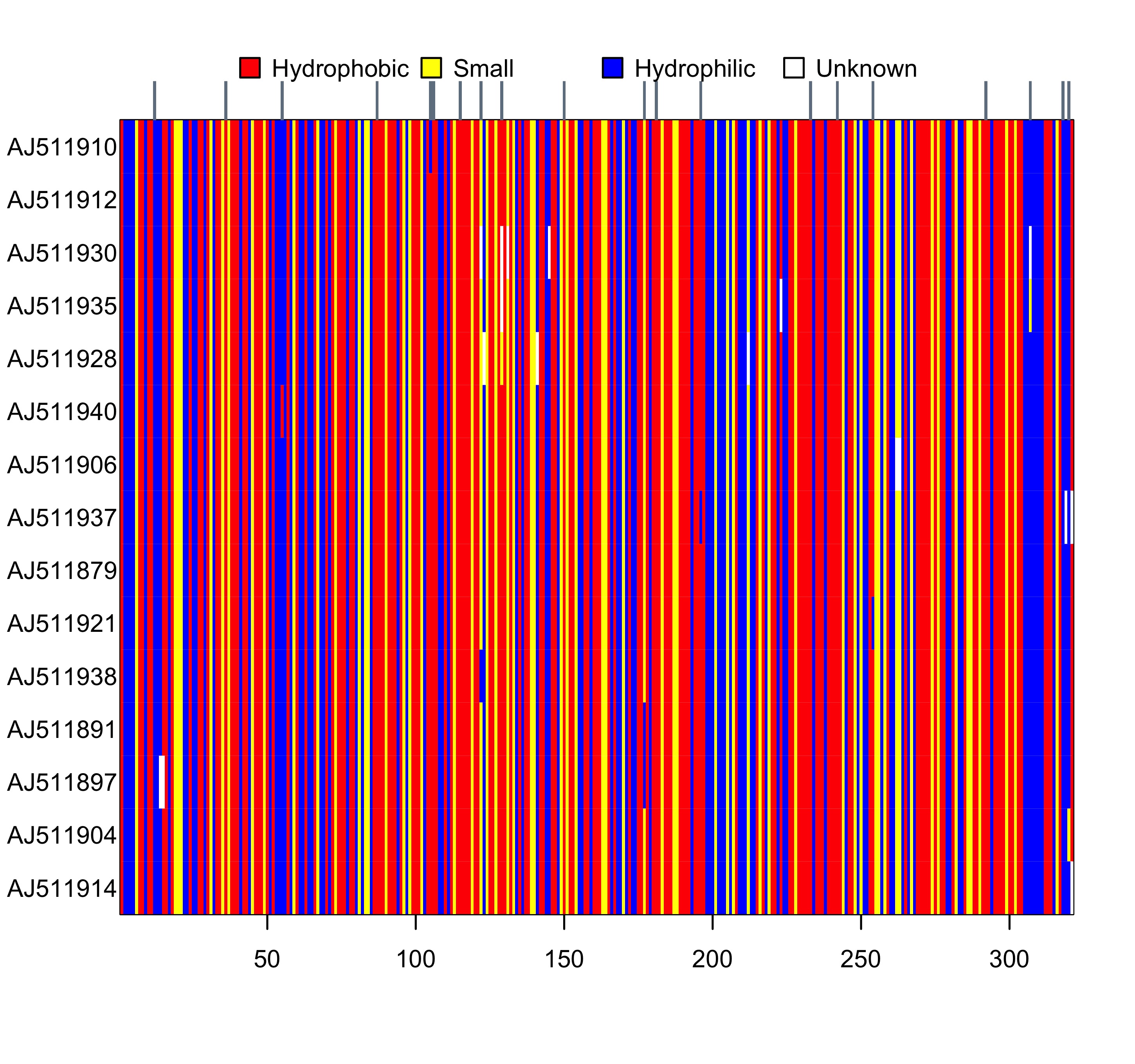
图 1: woodmouse_sel 翻译为氨基酸序列后的可视化结果
五、序列可视化
序列比对完成之后,使用image.DNAbin 可以对DNA序列可视化,使用 image.AAbin 函数可以对氨基酸序列可视化,对于核苷酸和氨基酸序列也可以直接用 image 函数。
### 显示缺失值为红色
image(woodmouse_sel_align, "n", "red")
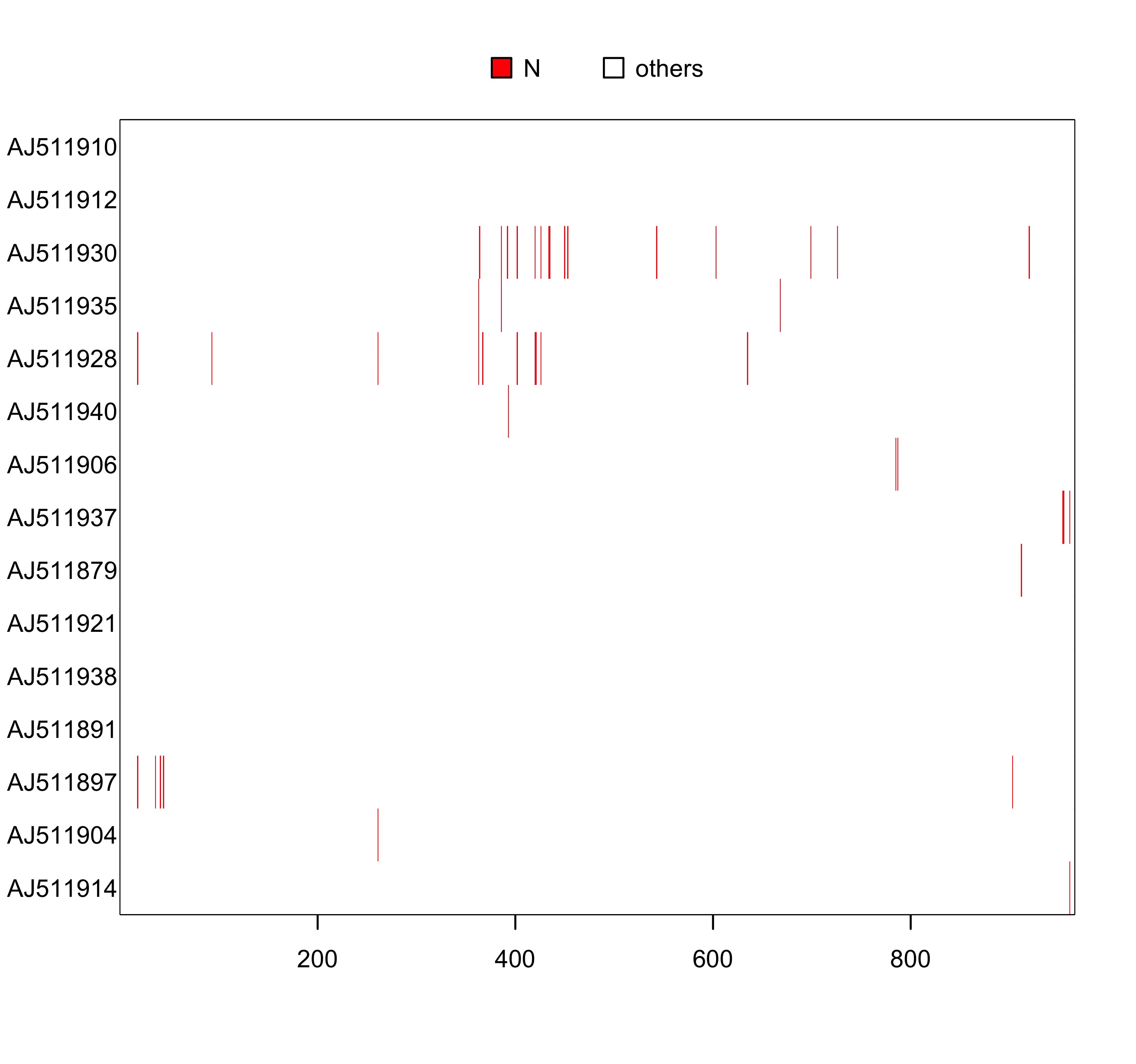
图 2: 序列 woodmouse_sel_align 的可视化,缺失位点用红色表示
### 显示 G+C 的值为蓝色
image(woodmouse_sel_align, c("g", "c"), "blue")
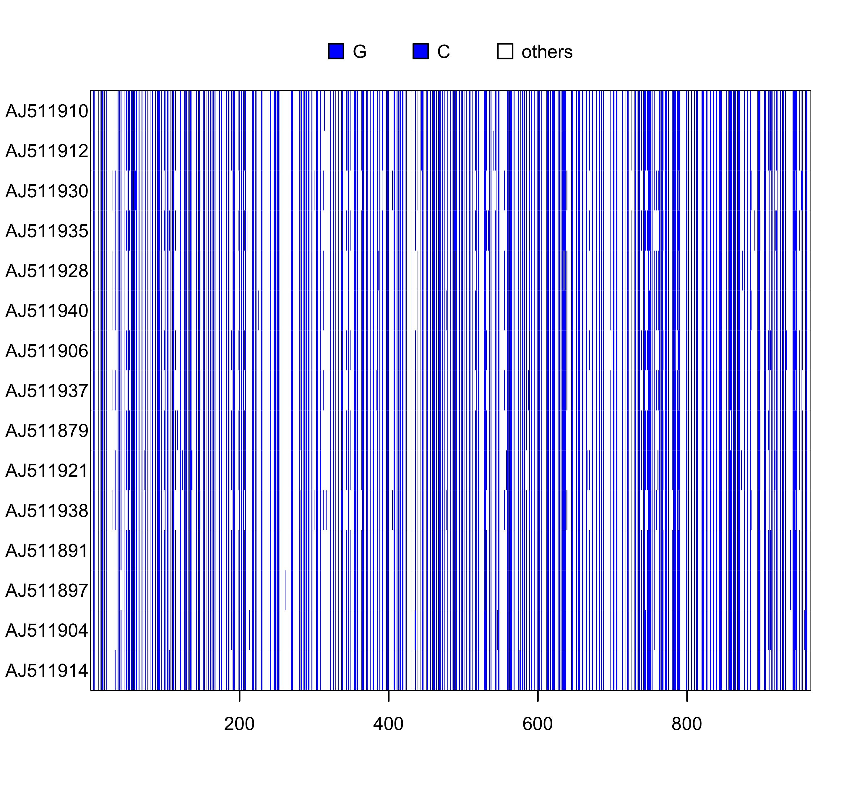
图 3: 序列 woodmouse_sel_align 的可视化, G+C 用蓝色表示
### 碱基 a 为 黑色
image(woodmouse_sel_align, "a", "black")
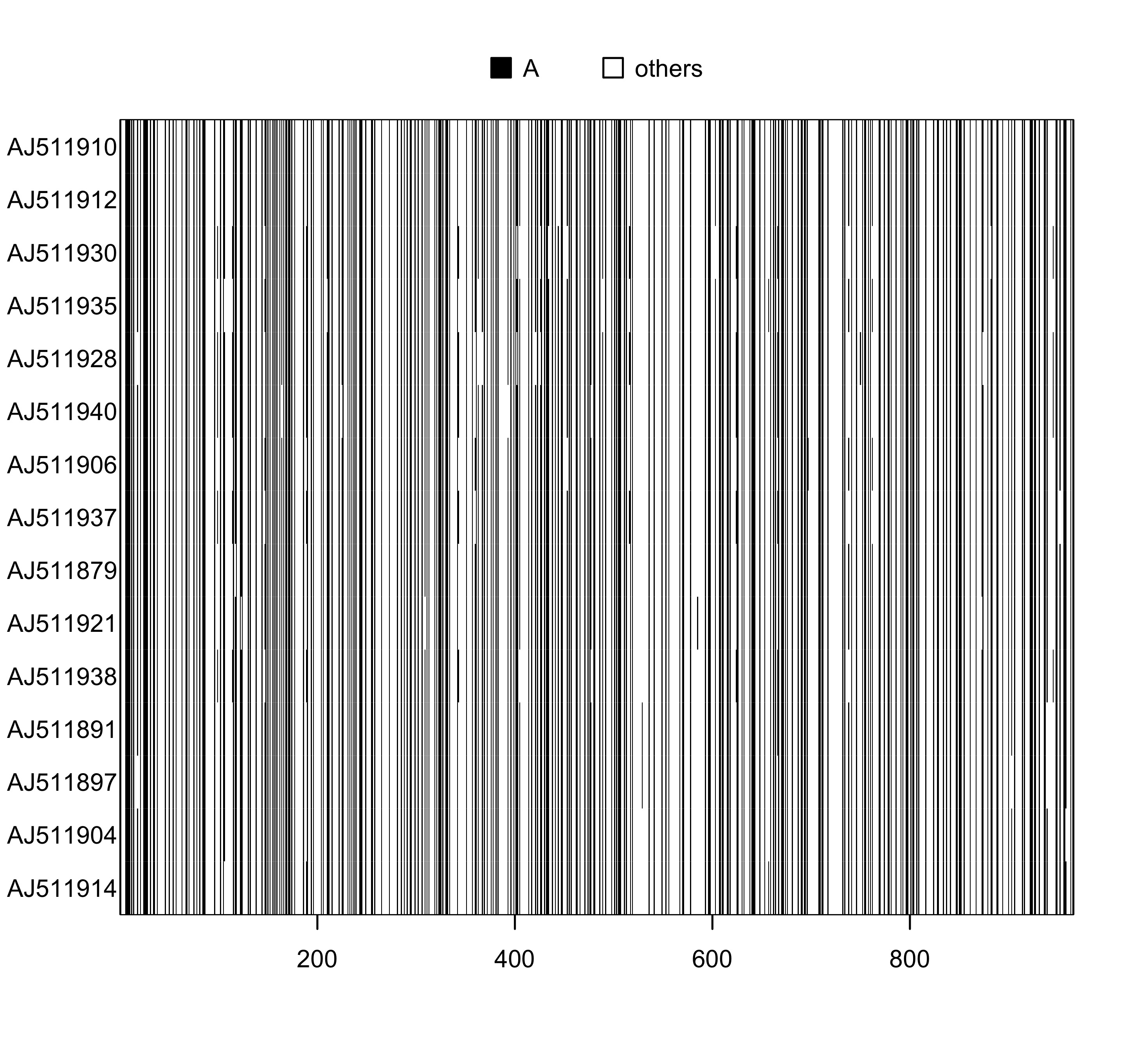
图 4: 序列 woodmouse_sel_align 的可视化, 碱基 A 用黑色表示
此外,用 all.equal 函数可以比较两条序列的差异。若选择 plot = FALSE 参数,则直接返回序列差异的比较结果(文字描述);若选择 plot = TRUE,则会用图形显示序列的差异。
### 定义 woodmouse_sel_align1 数据等于 woodmouse_sel_align 数据
woodmouse_sel_align1 <- woodmouse_sel_align
### 修改第一条序列1-10列的碱基为 “g”
woodmouse_sel_align1[1, c(1:10)] <- as.DNAbin("g")
all.equal(woodmouse_sel_align, woodmouse_sel_align1, plot = TRUE)

图 5: 序列差异的可视化结果
## $messages
## [1] "Labels in both objects identical."
##
## $different.sites
## [,1] [,2]
## [1,] 1 1
## [2,] 1 2
## [3,] 1 3
## [4,] 1 4
## [5,] 1 6
## [6,] 1 7
## [7,] 1 8
## [8,] 1 9
## [9,] 1 10
通过上图可以看出,all.equal 函数可以把序列有差异的列单独提取进行可视化,其他列则不再显示。
六、计算遗传距离
序列比对之后可以使用 dist.dna 函数计算成对比较遗传距离,模型选择会影响 dist.dna 的计算结果。本函数默认选择的模型是 “K80” (Kimura, 1980),此模型在DNA 条形码研究中经常用到。此外,对于存在缺失值的数据,pairwise.deletion 参数也会对结果有所影响。
models <- c("RAW", "JC69", "K80", "F81", "K81", "F84", "T92", "TN93", "GG95")
dist <- lapply(models, function(x) dist.dna(woodmouse_sel_align, model = x))
boxplot(dist, col = rainbow(9))

图 6: 不同模型下的遗传距离箱线图比较
七、构建进化树
- NJ 法
序列比对完成后,使用nj 函数可以基于遗传距离构建 NJ (neighbor-joining) 树. 此方法是 Saitou 和 Nei 于 1987年提出的,在DNA条形码研究中经常用到。
tree <- nj(dist.dna(woodmouse_sel_align))
plot(tree, edge.width = 1.5)

图 7: 展示进化树 tree
- bootstrap 分析
上面步骤计算得到的NJ树如果想要得到节点支持率可以使用 boot.phylo 函数,重抽样次数一般设置为1000。计算完节点支持率后可以使用 drawSupportOnEdges 函数将支持率添加到树的分支上。
### 定义 fun 函数
fun <- function(x) nj(dist.dna(x))
tree <- fun(woodmouse_sel_align)
set.seed(12345)
bp <- boot.phylo(tree, woodmouse_sel_align, fun, quiet = F, B = 1000)
##
Running bootstraps: 100 / 1000
Running bootstraps: 200 / 1000
Running bootstraps: 300 / 1000
Running bootstraps: 400 / 1000
Running bootstraps: 500 / 1000
Running bootstraps: 600 / 1000
Running bootstraps: 700 / 1000
Running bootstraps: 800 / 1000
Running bootstraps: 900 / 1000
Running bootstraps: 1000 / 1000
## Calculating bootstrap values... done.
plot(tree, edge.width = 1.5)
### 在分支上添加节点支持率
drawSupportOnEdges(round(bp/10, 0), cex = 0.8)

图 8: 展示进化树 tree,添加节点支持率
八、树的读取和写入 - 树的写入
树的写入可以使用的函数有 write.tree 和 write.nexus。write.tree 函数可以生成 Newick 格式树文件;write.nexus 则可生成 NEXUS 格式树文件。 在此我们可以把上面得到的进化树保存到本地。
### Newick 格式
write.tree(tree, file = "woodmouse_sel.tre")
### NEXUS 格式
write.nexus(tree, file = "woodmouse_sel.nex.tre")
- 树的读取
ape 有两个函数可以读取树文件,read.tree 和 read.nexus。 两个函数可以分别读取 Newick 和 NEXUS格式的树文件。我们可以用这两个函数读取刚才写入的两个树文件。
tree.nwk <- read.tree("woodmouse_sel.tre")
tree.nex <- read.nexus("woodmouse_sel.nex.tre")
plot(tree.nwk, edge.width = 1.5)
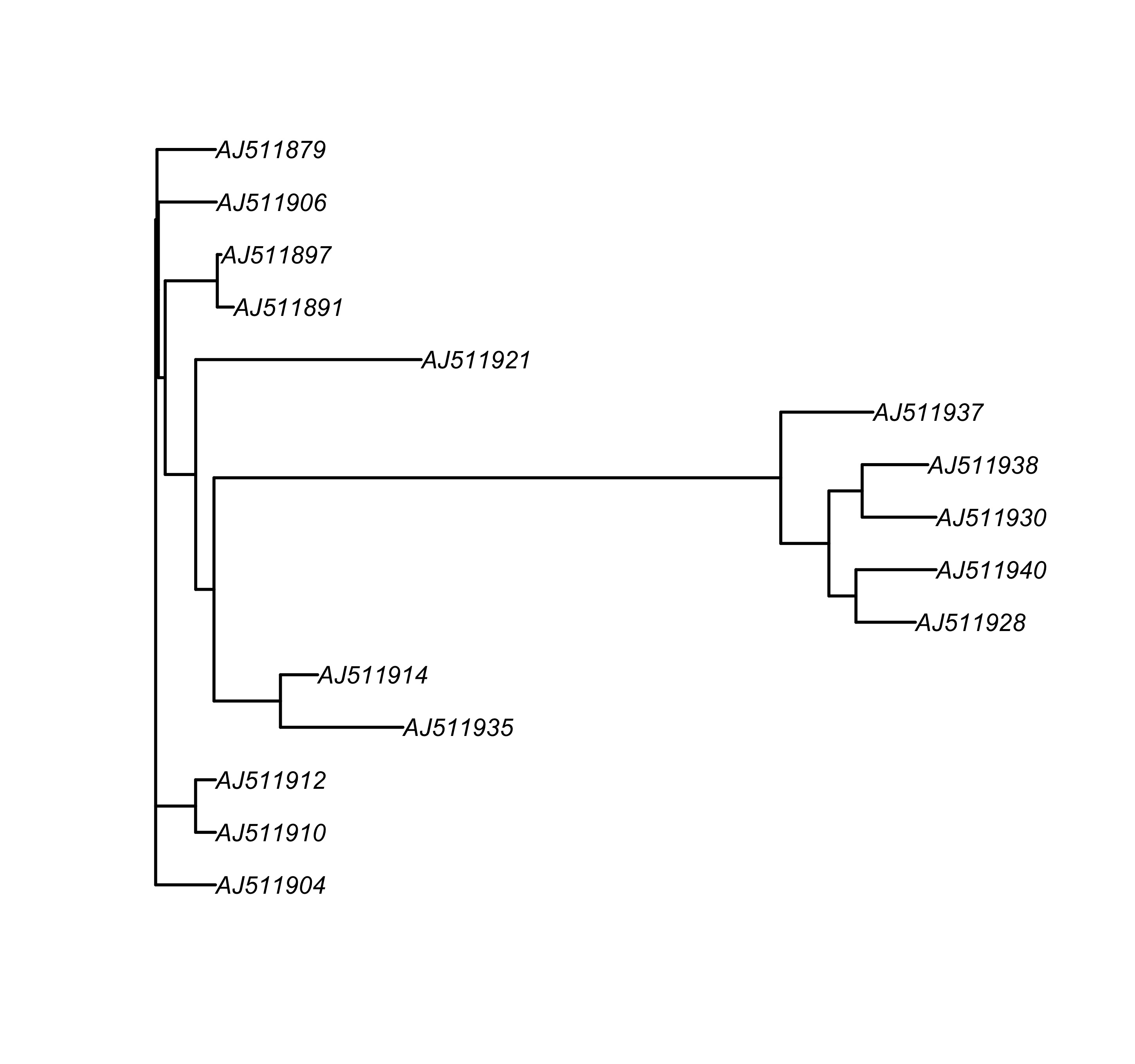
图 9: 展示进化树 tree.nwk
九、树的常见操作 - 置根
在 ape 包中可以使用 root 函数置根系统发育树。置根需要选择外群,在这里为了便于演示,暂用 “AJ511938” 进行置根。实际操作时,选择指定的外群进行置根即可。
tree_root <- root(tree, "AJ511938")
plot(tree_root, edge.width = 1.5)
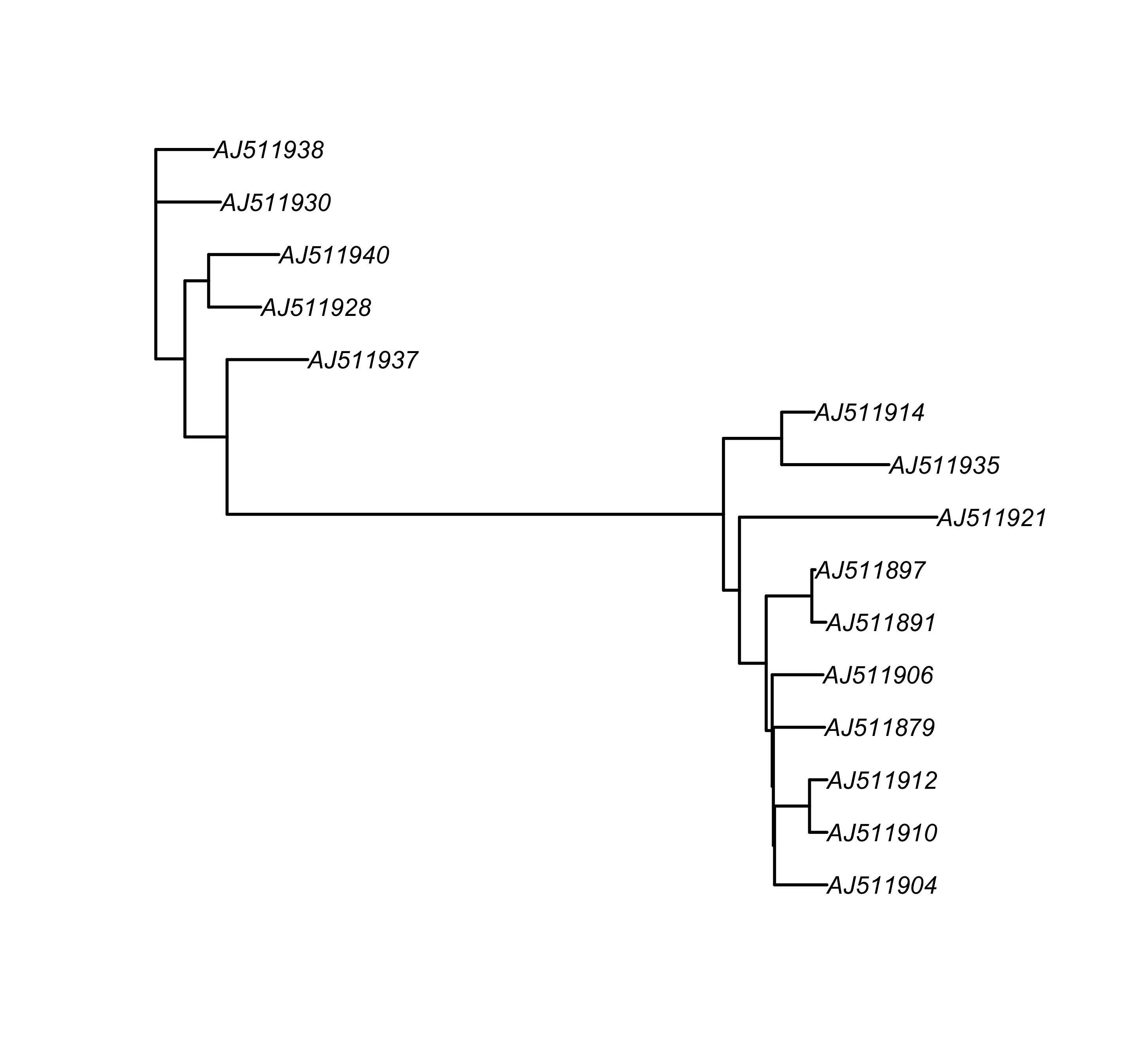
图 10: 展示置根后的进化树 tree_root
- 比较两个系统发育树的差异
对于两个系统发育树,尤其是类群比较多的情况下,直接观察不容易发现两者的区别。使用 comparePhylo 函数可以比较两个系统发育树的差异。若参数选择 plot = TRUE,则通过图形显示两者差异,反之则只使用文字进行描述。
a <- tree
### 去除两个末端节点
b <- drop.tip(tree, 1:2)
### 比较两棵树的差异
comparePhylo(a, b, plot = TRUE, force.rooted = TRUE)

图 11: 两棵树的差异比较
## => Comparing a with b.
## Trees have different numbers of tips: 15 and 13.
## Tips in a not in b : AJ511910, AJ511912.
## Trees have different numbers of nodes: 13 and 12.
## a is unrooted, b is rooted.
## Both trees are not ultrametric.
## 2 clades in a not in b.
## 1 clade in b not in a.
- 旋转一个节点的两个分支
ape 包还有一个实用的函数是 rotate 函数。使用 rotate 函数可以旋转一个节点的两个分支。
op <- par(no.readonly = TRUE)
par(mfrow = c(1, 2))
### 旋转第24个节点位置的末端标签
tree_rotate <- rotate(tree, 24)
plot(ladderize(tree), sub = "A")
nodelabels("", 24, frame = "c", bg = "red")
plot(ladderize(tree_rotate), sub = "B")
nodelabels("", 24, frame = "c", bg = "red")
par(op)

图 12: 比较进化树 tree 和 tree_rotate
通过上图可以看出红色节点位置(node = 24)的末端节点标签发生了互换。
- 系统发育树局部放大
对于类群数目比较多的系统发育树,使用 zoom 函数可以放大系统发育树的指定部分。若参数选择 subtree = FALSE,则不展示其他末端节点,反之则会将其他末端节点依次进行合并,只显示合并后的末端节点数目。
zoom(tree, 1:3, subtree = FALSE)

图 13: 树的局部放大,只显示放大部分
zoom(tree, 1:3, subtree = TRUE)

图 14: 树的局部放大,其他部分只显示末端节点数目
zoom(tree, grep("8", tree$tip.label), subtree = FALSE)

图 15: 树的局部放大,显示末端标签含有 “8” 的分支
- 去除系统发育树的末端节点
使用 drop.tip 函数可以去除系统发育树的末端节点。这里可以使用末端节点的编号,也可以直接输入末端节点的名称。
tree1 <- drop.tip(tree, 1:5, subtree = FALSE)
comparePhylo(tree, tree1, plot = FALSE)
## => Comparing tree with tree1.
## Trees have different numbers of tips: 15 and 10.
## Tips in tree not in tree1 : AJ511910, AJ511912, AJ511930, AJ511935, AJ511928.
## Trees have different numbers of nodes: 13 and 9.
## tree is unrooted, tree1 is rooted.
## Both trees are not ultrametric.
par(mfrow = c(1, 2))
plot(tree, main = "tree", sub = "A", edge.width = 1.5)
plot(tree1, main = "tree1", sub = "B", edge.width = 1.5)
par(op)

图 16: 展示去除特定末端节点后树形的变化
- 生成超度量树
为了推断分歧时间,需要把系统发育树转换为超度量树。在这里可以使用 chronos 函数,此函数可以使用 Penalised Likelihood (Sanderson, 2002; Kim and Sanderson, 2008) 和 Maximum Likelihood(Paradis, 2013)方法生成超度量树。为了便于演示,此处选择NJ树,实际使用时需要输入ML/BI树。
tree <- nj(dist.dna(woodmouse_sel, pairwise.deletion = TRUE))
str(tree)
## List of 4
## $ edge : int [1:27, 1:2] 16 16 19 21 23 24 24 23 25 26 ...
## $ edge.length: num [1:27] 0.004118 0.000615 0.002347 0.001033 0.003489 ...
## $ tip.label : chr [1:15] "AJ511910" "AJ511912" "AJ511930" "AJ511935" ...
## $ Nnode : int 13
## - attr(*, "class")= chr "phylo"
## - attr(*, "order")= chr "cladewise"
### 默认使用 correlated rate 模型
tree_chronos <- chronos(tree)
##
## Setting initial dates...
## Fitting in progress... get a first set of estimates
## (Penalised) log-lik = -0.5692622
## Optimising rates... dates... -0.5692622
## Warning: false convergence (8)
##
## log-Lik = -0.56827
## PHIIC = 79.14
tree$edge.length
## [1] 4.117731e-03 6.154783e-04 2.346552e-03 1.032984e-03 3.489051e-03
## [6] 6.447749e-03 1.939005e-03 2.990860e-02 2.562387e-03 1.265861e-03
## [11] 4.295423e-03 4.146896e-03 2.193855e-03 4.619535e-03 3.865063e-03
## [16] 4.689343e-03 1.173483e-02 2.515568e-03 7.214804e-05 1.991459e-04
## [21] 2.800554e-03 9.306119e-04 1.155711e-03 4.013051e-03 2.152766e-03
## [26] 1.038423e-03 1.038423e-03
plot(tree_chronos, edge.width = 1.5)

图 17: 展示超度量树 tree_chronos
- 多样性分析
生成超度量树之后,使用 ltt.plot 函数可以绘制 LTT 图形。LTT 图形可以描述支系随时间变化的趋势。
### 绘制LTT图
ltt.plot(tree_chronos)
title("Lineages Through Time Plot")

图 18: 使用ltt.plot函数绘制的LTT图
### 将树和 LTT 图形绘制在一起
par(mfrow = c(1, 2))
plot(tree_chronos, show.tip.label = TRUE, edge.width = 1.5)
ltt.plot(tree_chronos)
par(op)

图 19: 将树和 LTT 图共同展示
### 也可使用 ltt.coplot 函数
ltt.coplot(tree_chronos, show.tip.label = TRUE, x.lim = 1.1)
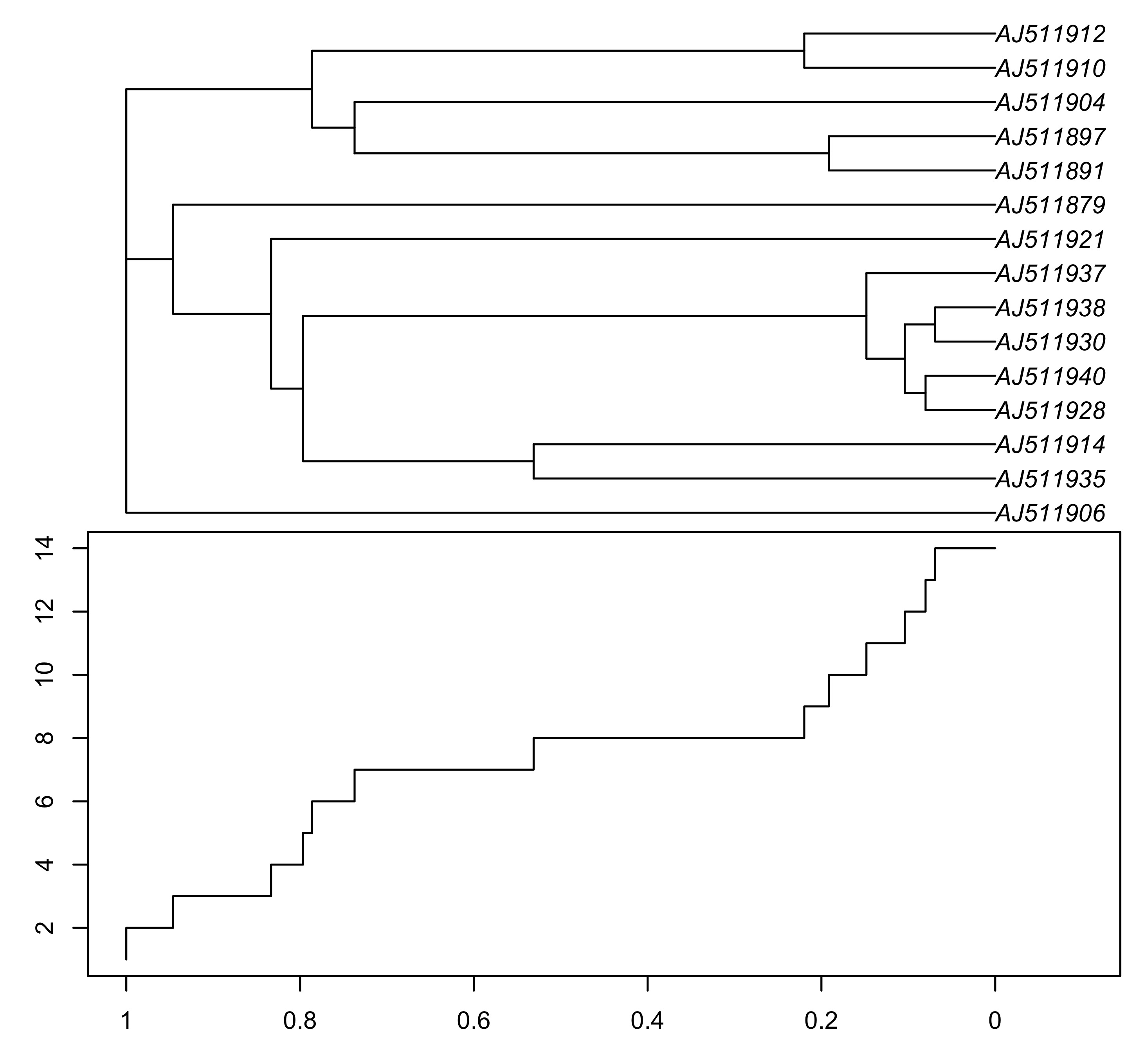
图 20: 使用ltt.plot函数绘制的LTT图
### 同时绘制多个 LTT 图形
par(mfrow = c(1, 1))
tree_chronos1 <- drop.tip(tree_chronos, 1:2)
tree_chronos2 <- drop.tip(tree_chronos, 3:4)
mltt.plot(tree_chronos, tree_chronos1, tree_chronos2)

图 21: 同时展示多个 LTT 图形
### 模拟数据,rcoal 函数可以随机生成超度量树
tree_rcoalx <- lapply(1:1000, function(x) rcoal(10))
mltt.plot(tree_rcoalx, legend = FALSE)

图 22: 同时展示1000个 LTT 图形
十、树的可视化
- 改变树的展示方式
ape 包的 plot.phylo 函数提供了系统发育树多种不同的展示方式,如下图所示:
par(mfrow = c(3, 2))
plot(tree, type = "p", main = "phylogram with branch lengths", sub = "A", use.edge.length = TRUE) # 默认
plot(tree, type = "p", main = "phylogram without branch lengths", sub = "B", use.edge.length = FALSE)
plot(tree, type = "c", main = "cladogram", sub = "C")
plot(tree, type = "f", main = "fan", sub = "D")
plot(tree, type = "u", main = "unrooted", sub = "E")
plot(tree, type = "r", main = "radial", sub = "F")
par(op)

图 23: 系统发育树六种不同的展示方式
- 末端标签对齐
使用 align.tip.label = TRUE,可以将系统发育树的末端标签进行对齐操作。
plot(tree, type = "p", align.tip.label = TRUE, edge.width = 1.5)

图 24: 系统发育树末端标签对齐
- 系统发育树的细节修改
系统发育树的细节修改包括线型、分支颜色和粗细等,可以根据具体要求进行调节。
### 改变分支的线型
par(mfrow = c(3, 2))
for (i in 1:6) {
plot(tree, edge.lty = i, sub = LETTERS[i], cex = 0.8)
}
par(op)
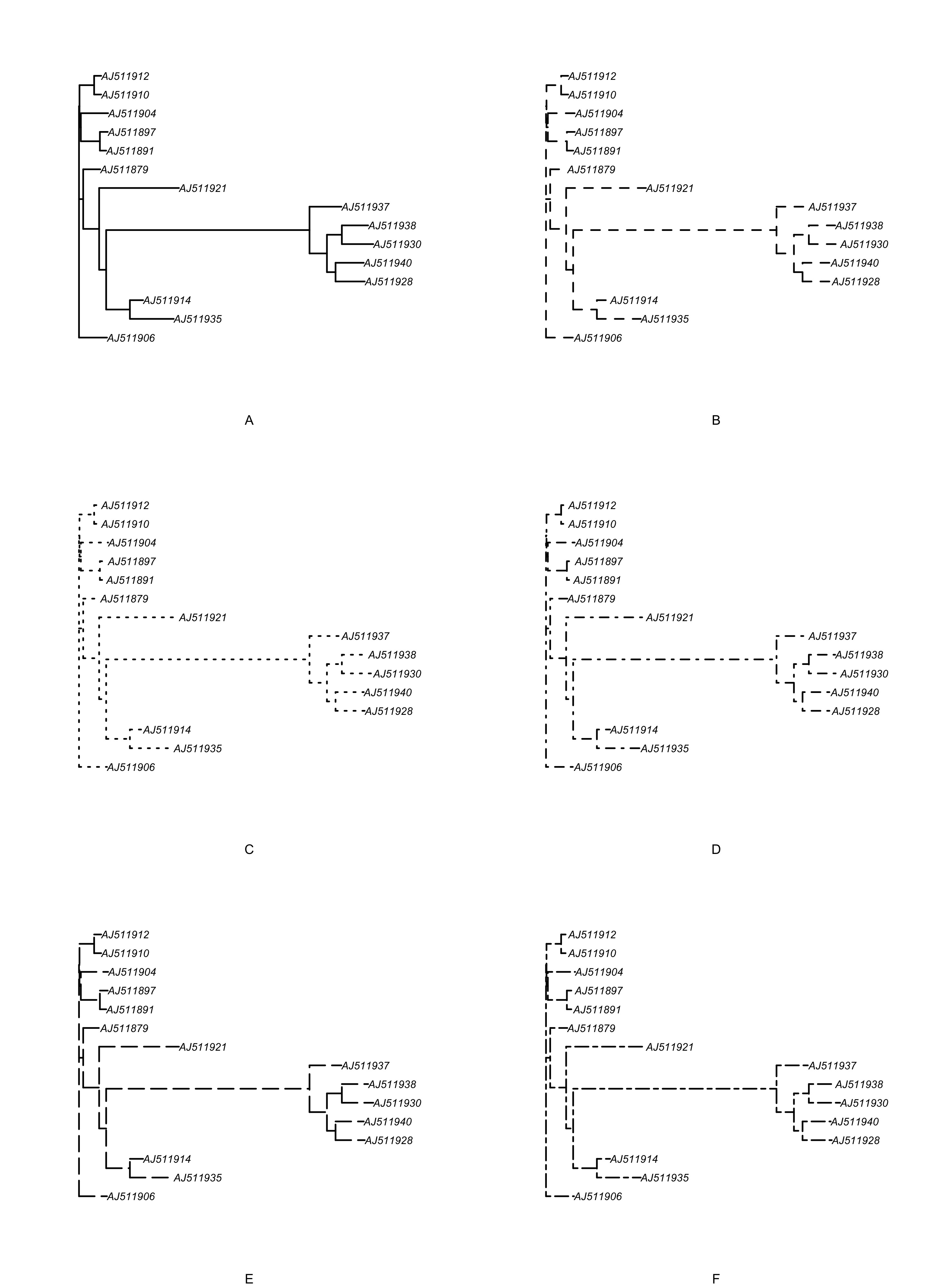
图 25: 比较系统发育树的六种线型
### 改变分支的颜色
plot(tree, edge.color = rainbow(27), edge.width = 1.5)

图 26: 改变系统发育树分支的颜色
### 改变分支的粗细
plot(tree, edge.width = 1:27/2)

图 27: 改变系统发育树分支的粗细
### 改变末端标签的颜色
plot(tree, tip.color = rainbow(15))

图 28: 改变系统发育树末端标签的颜色
### 改变字体 (默认斜体)
### font 的数值可选择1-4,分别代表常规字体,粗体,斜体,粗斜体。
par(mfrow = c(2, 2))
for (i in 1:4) {
plot(tree, font = i, sub = LETTERS[i], cex = 1.2)
}
par(op)

图 29: 改变系统发育树末端标签的字体
- 增加标签及注释
nodelabels 函数可以为系统发育树增加内部节点标签。
plot(tree, edge.width = 1.5)
nodelabels(bg = "lightgray", frame = "c")

图 30: 展示系统发育树的内部节点编号
### 加入节点标签
plot(tree, edge.width = 1.5)
nodelabels("circle", 17, frame = "c", bg = "red", adj = 0.5, cex = 0.6)
nodelabels("rect", 19, frame = "r", bg = "yellow", font = 1, adj = 0)

图 31: 展示系统发育树的特定节点标签
### 更改字体,为防止重叠可以使用 adj 参数进行调整
plot(tree, use.edge.length = FALSE, font = 1, edge.width = 1.5)
nodelabels(1:13, adj = -0.2, frame = "n", font = 1)
nodelabels(14:26, adj = c(1.2, 1), frame = "n", font = 2)
nodelabels(27:39, adj = c(1.2, -0.2), frame = "n", font = 3)

图 32: 树的每个内部节点同时显示3个数字
### 节点标签使用饼图
plot(tree, "c", use.edge.length = FALSE, edge.width = 1.5)
nodelabels(pie = runif(13), piecol = rainbow(3))

图 33: 树的节点标签使用饼图
### 节点标签使用柱状图
plot(tree, "c", use.edge.length = FALSE, edge.width = 1.5)
nodelabels(thermo = runif(13), piecol = rainbow(3))

图 34: 树的节点标签使用柱状图
### 节点标签使用水平柱状图
plot(tree, "c", use.edge.length = FALSE, edge.width = 1.5)
nodelabels(thermo = runif(13), piecol = rainbow(3), horiz = TRUE)

图 35: 树的节点标签使用水平柱状图
此外,祖先状态重建结果的可视化也需要用到 nodelabels 函数。
### 随机生成15个超度量树
tree_rcoal <- rcoal(15)
### rnorm(15) 可以生成符合正态分布的15个随机数 (mean = 0, sd = 1)
x <- rnorm(15)
### 生成离散型变量
x <- factor(c(rep(0, 5), rep(1, 10)))
ans <- ace(x, tree_rcoal, type = "d")
plot(tree_rcoal, type = "p", TRUE, edge.width = 1.5)
co <- c("red", "blue")
tiplabels(pch = 22, bg = co[as.numeric(x)], cex = 2, adj = 1)
nodelabels(thermo = ans$lik.anc, piecol = co, cex = 0.6)

图 36: 祖先特征重建结果
### 使用饼图
plot(tree_rcoal, edge.width = 1.5)
### 定义颜色
co <- c("red", "blue")
tiplabels(pch = 21, bg = "yellow", cex = 1.5, adj = 1)
nodelabels(pie = ans$lik.anc, piecol = co, cex = 0.6)

图 37: 祖先特征重建结果,使用饼图
使用 tiplabels 函数可以为系统发育树添加末端节点标签。
### 显示末端节点编号
plot(tree, edge.width = 1.5)
tiplabels()

图 38: 展示系统发育树的末端节点编号
plot(tree, "p", use.edge.length = FALSE, edge.width = 1.5, label.offset = 3, x.lim = 31)
tiplabels(pch = 18, col = gray.colors(13), cex = 3, adj = 1.4)
tiplabels(pch = 19, col = rainbow(13), adj = 2.5, cex = 3)

图 39:树的末端同时展示两种不同的特征
使用 edgelabels 函数可以在系统发育树的分支上添加标签。
plot(tree, edge.width = 1.5)
edgelabels()

图 40: 展示树的分支编号
plot(tree, edge.width = 1.5)
edgelabels(round(tree$edge.length, 3), srt = 0)

图 41: 在树的分支中展示支长
plot(tree, "p", FALSE, edge.width = 1.5)
edgelabels("a", adj = c(0.5, -0.25), bg = "grey")
edgelabels("b", adj = c(0.5, 1.25), bg = "white")

图 42: 在树的分支上下添加文字
- 添加坐标轴
使用 axisPhylo 函数可以为系统发育树添加坐标轴。
par(mfrow = c(1, 2))
plot(tree, edge.width = 1.5, sub = "A")
axisPhylo()
plot(tree, direction = "u", edge.width = 1.5, sub = "B")
### 改变方向
axisPhylo(2, las = 1)
par(op)

图 43: 添加坐标轴并改变方向
- 添加比例尺
使用 add.scale.bar 函数可以添加比例尺。add.scale.bar 函数也可以定义比例尺的字号、字体和颜色。
### 自定义比例尺的字体和颜色
plot(tree, edge.width = 1.5)
add.scale.bar(cex = 1, font = 2, col = "red")

图 44: 为系统发育树添加比例尺
- 组合图形
cophyloplot 将两个系统发育树绘制在一起,同时将相同的末端标签用线段连接。
### 生成两个随机树
tree1 <- tree
tree2 <- drop.tip(tree, 1:5, subtree = FALSE)
### 生成相关矩阵
association <- cbind(tree2$tip.label, tree2$tip.label)
cophyloplot(tree1, tree2, assoc = association, length.line = 1, space = 30, gap = 2)
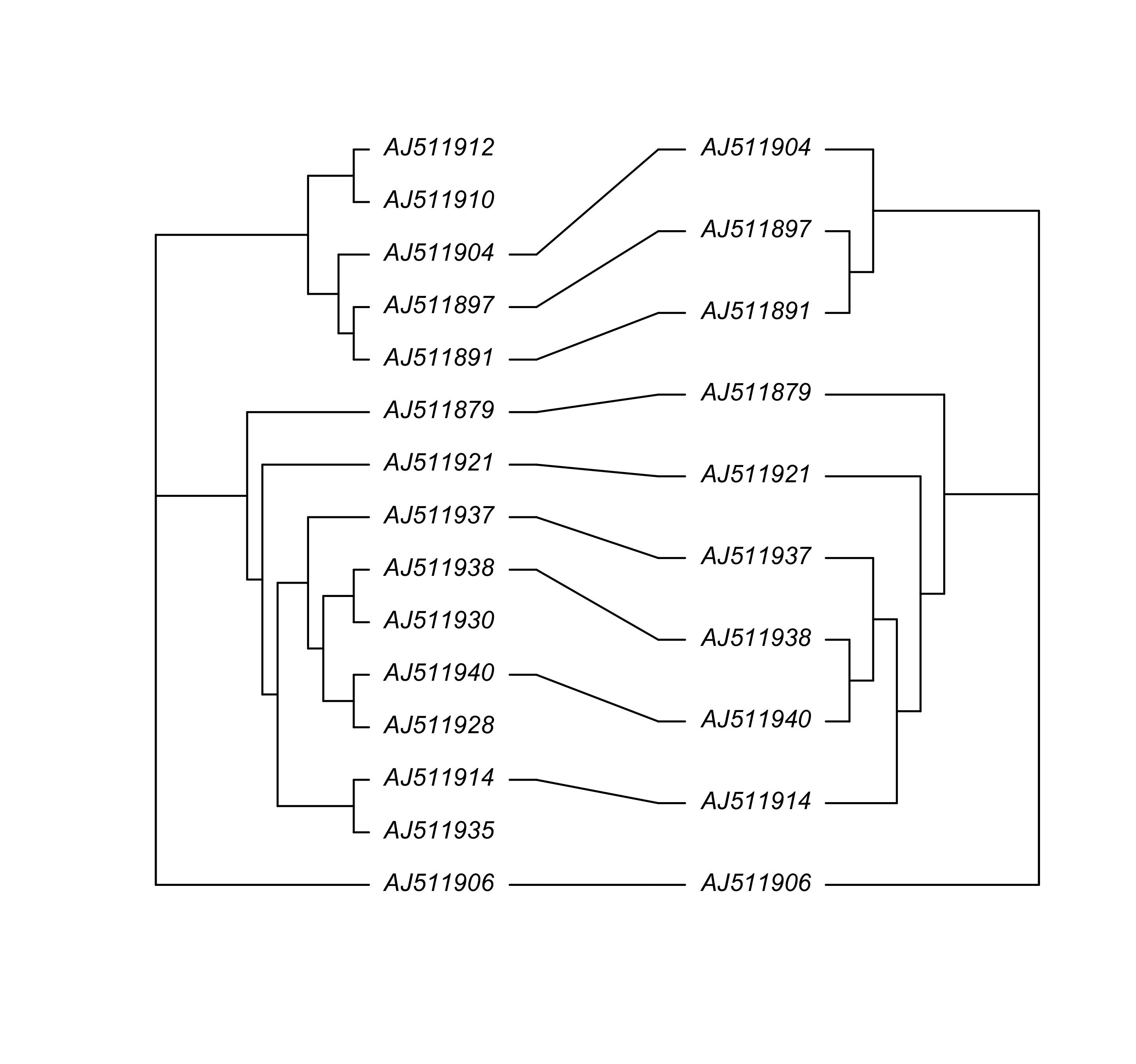
图 45: 同时展示 tree1和 tree2
另外,通过改变 direction 的参数,可以改变系统发育树的展示方向。比如可以使系统发育树进行左右或上下组合。
par(mfrow = c(2, 2))
plot(tree, "p", FALSE, direction = "r", sub = "A", edge.width = 1.5)
plot(tree, "p", FALSE, direction = "l", sub = "B", edge.width = 1.5)
plot(tree, "c", FALSE, direction = "u", sub = "C", edge.width = 1.5)
plot(tree, "c", FALSE, direction = "d", sub = "D", edge.width = 1.5)
par(op)

图 46: 改变树的方向
- 将树和图形共同展示
phydataplot 函数可以将树和图形进行组合,可供选择的类型有7种。
### 生成随机树,使展示的变量和树的标签对应
x <- 1:15
tree <- nj(dist.dna(woodmouse_sel_align, pairwise.deletion = TRUE))
tree_chronos <- chronos(tree)
##
## Setting initial dates...
## Fitting in progress... get a first set of estimates
## (Penalised) log-lik = -0.5692622
## Optimising rates... dates... -0.5692622
## Warning: false convergence (8)
##
## log-Lik = -0.56827
## PHIIC = 79.14
names(x) <- tree_chronos$tip.label
### 类型选择 'bars'
plot(tree_chronos, x.lim = 6, edge.width = 1.5)
phydataplot(x, tree_chronos, "bars", scaling = 0.25)

图 47: 将树和柱状图共同展示
### 类型选择 “segments”
plot(tree_chronos, x.lim = 6, edge.width = 1.5)
phydataplot(x, tree_chronos, "s", lwd = 3, lty = 3, scaling = 0.25)

图 48: 将树和线段共同展示
### 类型选择 “arrows”
plot(tree_chronos, x.lim = 6, edge.width = 1.5)
phydataplot(x, tree_chronos, "a", scaling = 0.25)

图 49: 将树和箭头共同展示
### 类型选择 “dotchart”
plot(tree_chronos, x.lim = 6, edge.width = 1.5)
phydataplot(x, tree_chronos, "d", scaling = 0.25)

图 50: 将树和点图共同展示
### 同时展示柱状图和点图
plot(tree_chronos, x.lim = 20, edge.width = 1.5)
phydataplot(x, tree_chronos, col = "yellow", scaling = 0.5, offset = 3)
phydataplot(x, tree_chronos, "d", scaling = 0.5, offset = 12)

图 51: 同时展示柱状图和点图
### runif 函数可以生成均匀分布的随机数
x <- runif(15, 0, 0.5)
y <- runif(15, 0, 0.5)
z <- 1 - x - y
m <- cbind(x, y, z)
rownames(m) <- tree_chronos$tip.label
plot(tree_chronos, x.lim = 3, edge.width = 1.5)
col <- c("red", "green", "blue")
phydataplot(m, tree_chronos, col = col, offset = 0.5)

图 52: 将树和堆积柱状图共同展示
### 生成矩阵
m <- matrix(rnorm(15 * 5), 15)
rownames(m) <- tree_chronos$tip.label
plot(tree_chronos, x.lim = 3, edge.width = 1.5)
### 展示箱线图
phydataplot(m, tree_chronos, "bo", scaling = 0.25, offset = 0.5, boxfill = c("red",
"skyblue"))

图 53: 将树和箱线图共同展示
### 在树的旁边显示序列联配结果
plot(tree_chronos, x.lim = 6, align.tip = FALSE, font = 1, edge.width = 1.5)
phydataplot(woodmouse_sel_align[, 1:100], tree_chronos, "m", scaling = 1, border = NA)

图 54: 将树和序列联配结果共同展示
dist <- dist.dna(woodmouse_sel_align)
par(mar = rep(1, 4))
plot(tree_chronos, x.lim = 5, cex = 0.8, font = 1)
phydataplot(as.matrix(dist), tree_chronos, "i", offset = 0.8)
par(op)

图 55: 将树和热图共同展示
此外,对于系统发育树的可视化,推荐使用 R 包 ggtree(Yu et al., 2017, Methods in Ecology and Evolution), 其使用方法详见 https://guangchuangyu.github.io/ggtree-book/chapter-ggtree.html。
致谢
感谢bio-protocol 的编辑工作以及两位匿名审稿专家提出建设性的修改意见。
参考文献
- Edgar, R. C. (2004) MUSCLE: Multiple sequence alignment with high accuracy and high throughput. Nucleic Acids Res 32: 1792-1797.
- Kimura, M. (1980). A simple method for estimating evolutionary rates of base substitutions through comparative studies of nucleotide sequences. J Mol Evol 16: 111-120.
- Kim, J. and Sanderson, M. J. (2008) Penalized likelihood phylogenetic inference: bridging the parsimony-likelihood gap. Syst Biol 57: 665-674.
- Michaux, J. R., Magnanou, E., Paradis, E., Nieberding, C. and Libois, R. (2003) Mitochondrial phylogeography of the Woodmouse (Apodemus sylvaticus) in the Western Palearctic region. Mol Ecol 12: 685-697.
- Paradis, E. and Schliep, K. (2019). ape 5.0: an environment for modern phylogenetics and evolutionary analyses in R. Bioinformatics 35(3): 526-528.
- Paradis, E. (2012) Developing and Implementing Phylogenetic Methods in R. In: Analysis of Phylogenetics and Evolution with R. Use R!. Springer, New York, NY.
- Paradis, E. (2013) Molecular dating of phylogenies by likelihood methods: a comparison of models and a new information criterion. Mol Phylogenet Evol 67: 436-444.
- Paradis, E., Claude, J. and Strimmer, K. (2004). APE: Analyses of Phylogenetics and Evolution in R language. Bioinformatics 20(2): 289-290.
- Saitou, N. and Nei, M. (1987) The neighbor-joining method: a new method for reconstructing phylogenetic trees. Mol Biol Evol 4: 406-425.
- Sanderson, M. J. (2002) Estimating absolute rates of molecular evolution and divergence times: a penalized likelihood approach. Mol Biol Evol 19: 101-109.
- Yu, G., Smith, D. K., Zhu, H., Guan, Y. and Lam, T.T.‐Y. (2017), GGTREE: an R package for visualization and annotation of phylogenetic trees with their covariates and other associated data. Methods Ecol Evol. 8(1): 28-36.